


GATE 2022 Statistics (ST) Question Paper with Solutions PDFs can be downloaded from this page. GATE 2022 was successfully conducted by IIT Kharagpur on 6th February, 2022. The exam was conducted in the Forenoon Session (9:00 AM to 12:00 PM). The question paper comprises two sections i.e. General Aptitude and Statistics based questions. 15% the total weightage was carried by General Aptitude. Statistics based questions carried the remaining 85% of the total weightage.
GATE 2022 Statistics (ST) Question Paper with Solutions
Candidates targeting GATE can download the PDFs for GATE 2022 ST Question Paper and Solutions to know the important topics asked, and check their preparation level by solving the past question papers.
| GATE 2022 Statistics (ST) Question Paper | Check Solutions |

Mr. X speaks _____ Japanese _____ Chinese.
A sum of money is to be distributed among P, Q, R, and S in the proportion 5 : 2 : 4 : 3, respectively.
If R gets ₹1000 more than S, what is the share of Q (in ₹)?
A trapezium has vertices marked as P, Q, R, and S (in that order anticlockwise). The side PQ is parallel to side SR. Further, it is given that, PQ = 11 cm, QR = 4 cm, RS = 6 cm, and SP = 3 cm. What is the shortest distance between PQ and SR (in cm)?
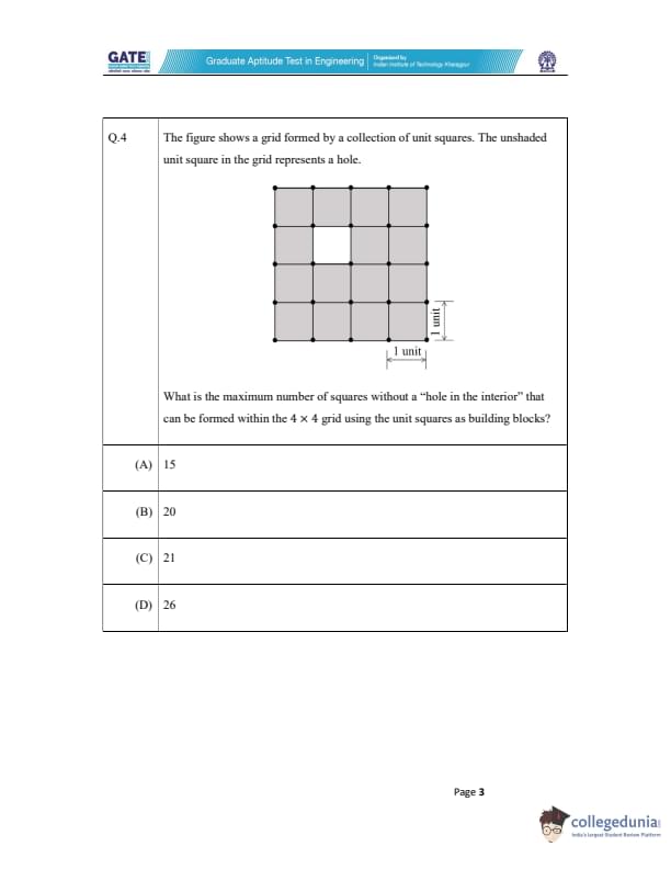
The figure shows a grid formed by a collection of unit squares. The unshaded unit square in the grid represents a hole. What is the maximum number of squares without a "hole in the interior" that can be formed within the 4 \(\times\) 4 grid using the unit squares as building blocks?

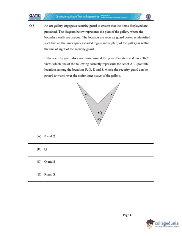
An art gallery engages a security guard to ensure that the items displayed are protected. The diagram below represents the plan of the gallery where the boundary walls are opaque. The location the security guard posted is identified such that all the inner space (shaded region in the plan) of the gallery is within the line of sight of the security guard.
If the security guard does not move around the posted location and has a 360° view, which one of the following correctly represents the set of ALL possible locations among the locations P, Q, R and S, where the security guard can be posted to watch over the entire inner space of the gallery?

Mosquitoes pose a threat to human health. Controlling mosquitoes using chemicals may have undesired consequences. In Florida, authorities have used genetically modified mosquitoes to control the overall mosquito population. It remains to be seen if this novel approach has unforeseen consequences.
Which one of the following is the correct logical inference based on the information in the above passage?
Consider the following inequalities.
(i) 2x - 1 \(>\) 7
(ii) 2x - 9 \(<\)1
Which one of the following expressions below satisfies the above two inequalities?
Four points \( P(0, 1), Q(0, -3), R(-2, -1), \) and \( S(2, -1) \) represent the vertices of a quadrilateral. What is the area enclosed by the quadrilateral?
In a class of five students P, Q, R, S and T, only one student is known to have copied in the exam. The disciplinary committee has investigated the situation and recorded the statements from the students as given below.
Statement of P: R has copied in the exam.
Statement of Q: S has copied in the exam.
Statement of R: P did not copy in the exam.
Statement of S: Only one of us is telling the truth.
Statement of T: R is telling the truth.
The investigating team had authentic information that S never lies.
Based on the information given above, the person who has copied in the exam is:
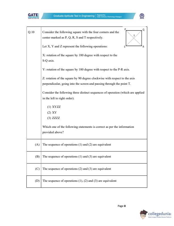
Consider the following square with the four corners and the center marked as P, Q, R, S and T respectively.
Let X, Y, and Z represent the following operations:
X: rotation of the square by 180 degree with respect to the S-Q axis.
Y: rotation of the square by 180 degree with respect to the P-R axis.
Z: rotation of the square by 90 degree clockwise with respect to the axis perpendicular, going into the screen and passing through the point T.
Consider the following three distinct sequences of operation (which are applied in the left to right order).
(1) XYZ
(2) XY
(3) ZZZZ
Which one of the following statements is correct as per the information provided above?

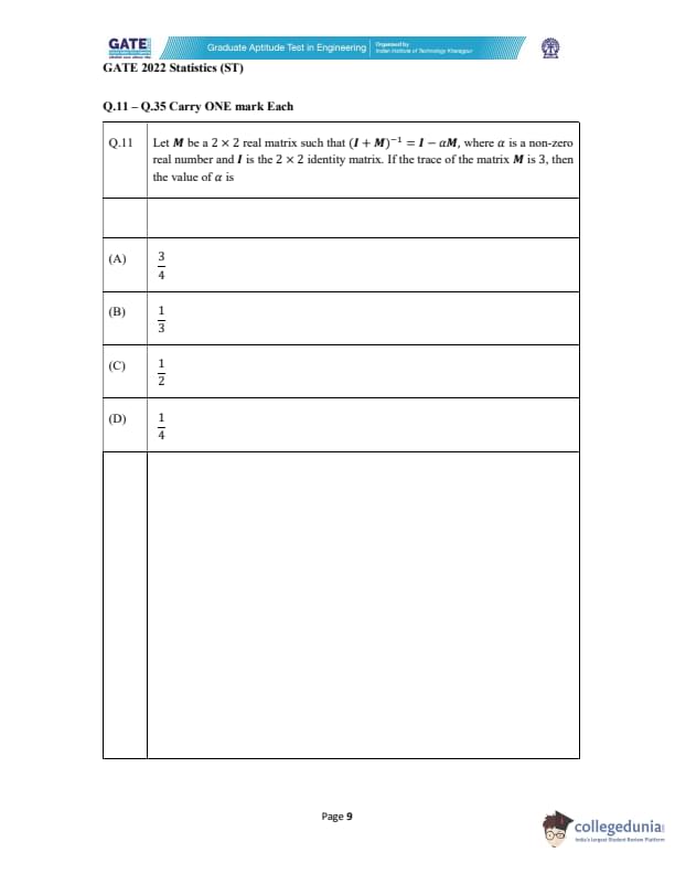
Let \(M\) be a 2 \(\times\) 2 real matrix such that \((I + M)^{-1} = I - \alpha M\), where \(\alpha\) is a non-zero real number and \(I\) is the 2 \(\times\) 2 identity matrix. If the trace of the matrix \(M\) is 3, then the value of \(\alpha\) is
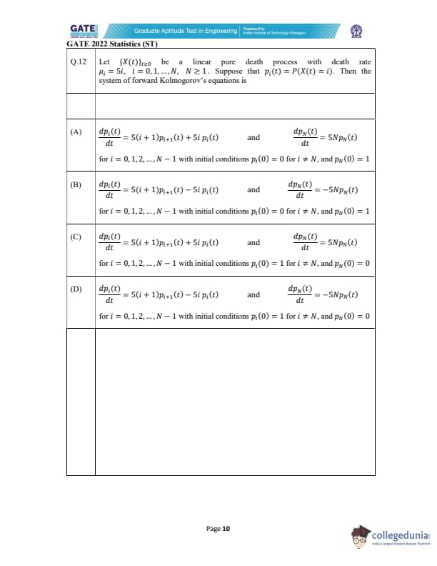
Let \(\{X(t)\}_{t\geq 0}\) be a linear pure death process with death rate \(\mu_i = 5i\), \(i = 0, 1, \dots, N\), \(N \geq 1\). Suppose that \(p_i(t) = P(X(t) = i)\). Then the system of forward Kolmogorov’s equations is
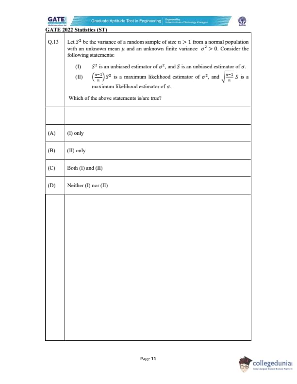
Let \( S^2 \) be the variance of a random sample of size \( n > 1 \) from a normal population with an unknown mean \( \mu \) and an unknown finite variance \( \sigma^2 > 0 \). Consider the following statements:
(I) \( S^2 \) is an unbiased estimator of \( \sigma^2 \), and \( S \) is an unbiased estimator of \( \sigma \).
(II) \( \frac{n-1}{n} S^2 \) is a maximum likelihood estimator of \( \sigma^2 \), and \( \sqrt{\frac{n-1}{n}} S \) is a maximum likelihood estimator of \( \sigma \).
Which of the above statements is/are true?
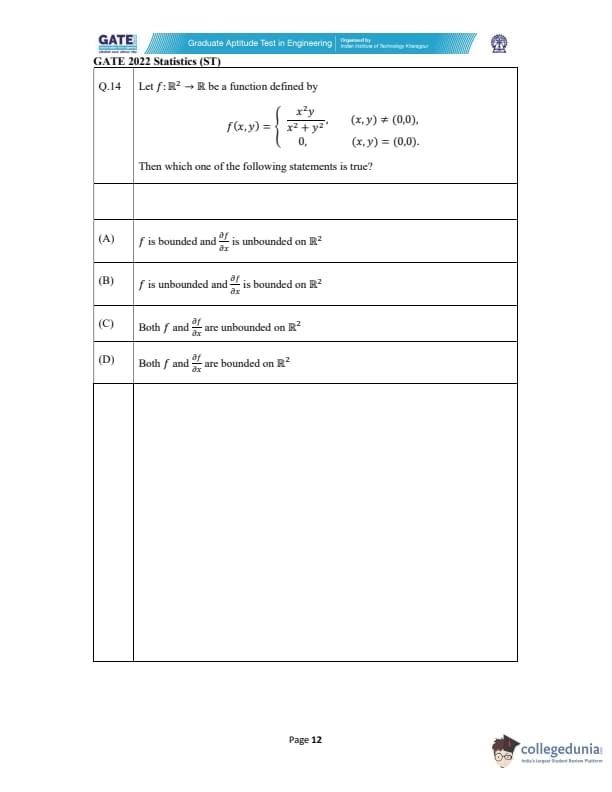
Let \( f : \mathbb{R}^2 \to \mathbb{R} \) be a function defined by \[ f(x, y) = \begin{cases} \frac{x^2 y}{x^2 + y^2} & if (x, y) \neq (0, 0),
0 & if (x, y) = (0, 0). \end{cases} \]
Find the value of \( \frac{\partial f}{\partial x} \) at \( (0, 0) \).
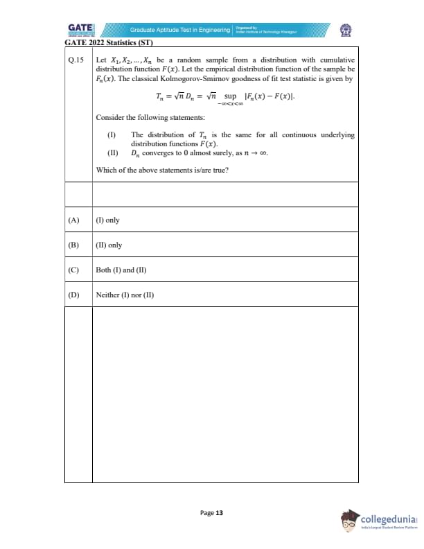
Let \( X_1, X_2, \dots, X_n \) be a random sample from a distribution with cumulative distribution function \( F(x) \). Let the empirical distribution function of the sample be \( F_n(x) \). The classical Kolmogorov-Smirnov goodness of fit test statistic is given by \[ T_n = \sqrt{n} D_n = \sqrt{n} \sup_{-\infty < x < \infty} | F_n(x) - F(x) |. \]
Consider the following statements:
The distribution of \( T_n \) is the same for all continuous underlying distribution functions \( F(x) \).
\( D_n \) converges to 0 almost surely, as \( n \to \infty \).
Which one of the following statements is/are true?
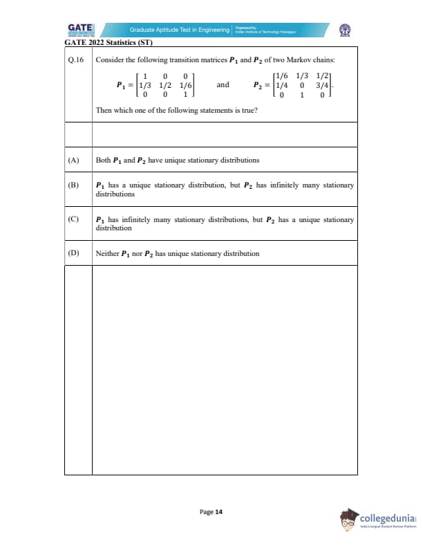
Consider the following transition matrices \( P_1 \) and \( P_2 \) of two Markov chains:

Which of the following statements is correct?
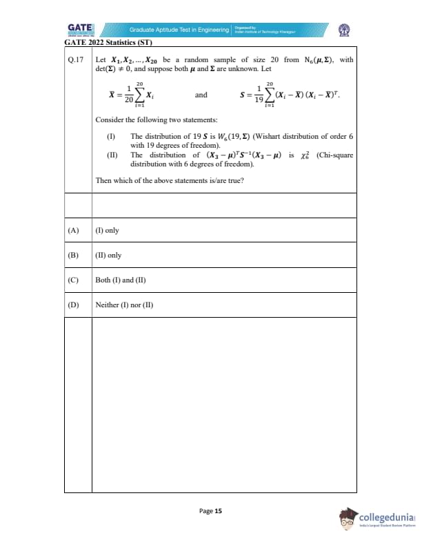
Let \( X_1, X_2, \dots, X_{20} \) be a random sample of size 20 from \( N_6(\mu, \Sigma) \), with det(\(\Sigma\)) \(\neq 0\), and suppose both \(\mu\) and \(\Sigma\) are unknown. Let \[ \bar{X} = \frac{1}{20} \sum_{i=1}^{20} X_i \quad and \quad S = \frac{1}{19} \sum_{i=1}^{20} (X_i - \bar{X})(X_i - \bar{X})^T. \]
Consider the following two statements:
The distribution of \( 19S \) is \( W_6(19, \Sigma) \) (Wishart distribution of order 6 with 19 degrees of freedom).
The distribution of \( (X_3 - \mu)^T S^{-1} (X_3 - \mu) \) is \( \chi^2_6 \) (Chi-square distribution with 6 degrees of freedom).
Then which of the above statements is/are true?
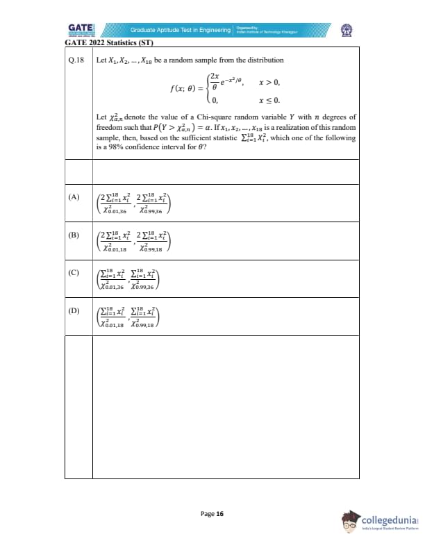
Let \( X_1, X_2, \dots, X_{18} \) be a random sample from the distribution \[ f(x; \theta) = \begin{cases} \frac{2x}{\theta} e^{-x^2/\theta}, & x > 0,
0, & x \leq 0. \end{cases} \]
What is the maximum likelihood estimator (MLE) of \( \theta \)?
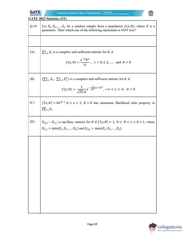
Let \( X_1, X_2, \dots, X_n \) be a random sample from a population \( f(x; \theta) \), where \( \theta \) is a parameter. Then which one of the following statements is NOT true?
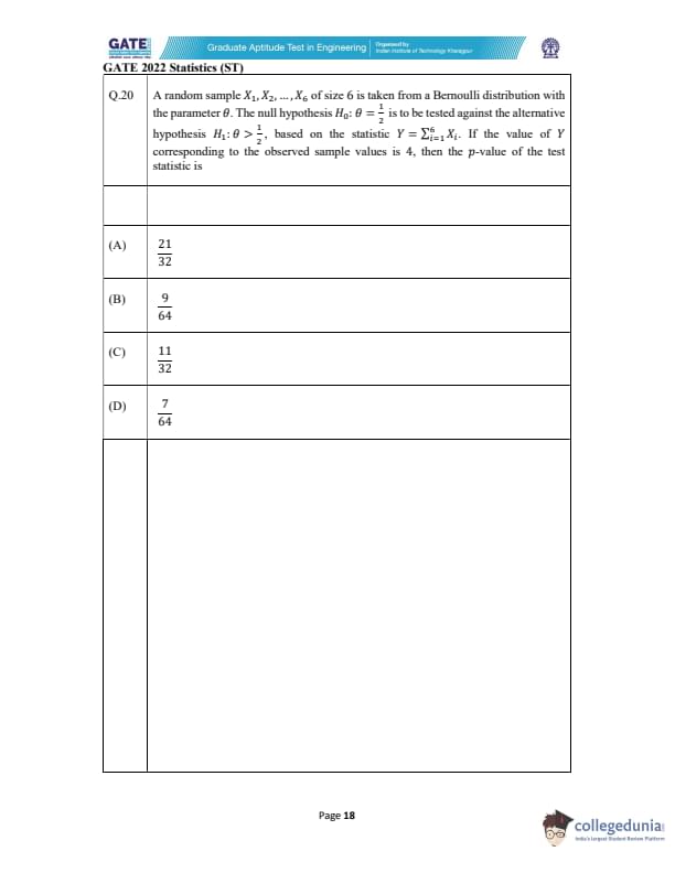
A random sample \( X_1, X_2, \dots, X_6 \) is taken from a Bernoulli distribution with the parameter \( \theta \). The null hypothesis \( H_0: \theta = \frac{1}{2} \) is to be tested against the alternative hypothesis \( H_1: \theta > \frac{1}{2} \), based on the statistic \( Y = \sum_{i=1}^{6} X_i \). If the value of \( Y \) corresponding to the observed sample values is 4, then the p-value of the test is ____?
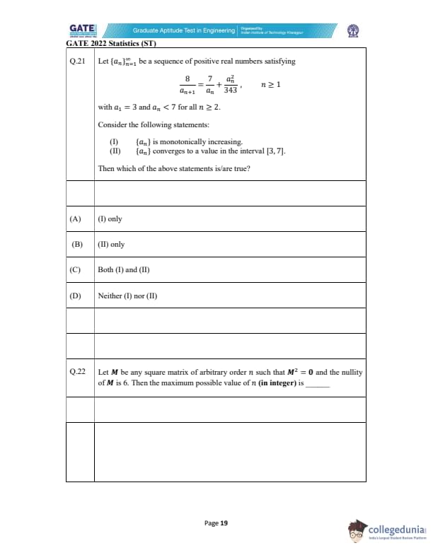
Let \(\{a_n\}_{n=1}^\infty\) be a sequence of positive real numbers satisfying \[ \frac{8}{a_{n+1}} = \frac{7}{a_n} + \frac{a_n^2}{343}, \quad n \geq 1, \]
with \(a_1 = 3\) and \(a_n < 7\) for all \(n \geq 2\).
Consider the following statements:
[(I)] \(\{a_n\}\) is monotonically increasing.
[(II)] \(\{a_n\}\) converges to a value in the interval \([3, 7]\).
Then which of the above statements is/are true?
Let \( M \) be any square matrix of arbitrary order \( n \) such that \( M^2 = 0 \) and the nullity of \( M \) is 6. Then the maximum possible value of \( n \) (in integer) is ________
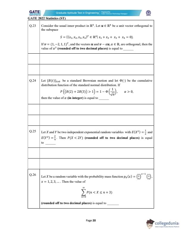
Consider the usual inner product in \( \mathbb{R}^4 \). Let \( u \in \mathbb{R}^4 \) be a unit vector orthogonal to the subspace \[ S = \{(x_1, x_2, x_3, x_4)^T \in \mathbb{R}^4 \mid x_1 + x_2 + x_3 + x_4 = 0 \}. \]
If \( v = (1, -2, 1, 1)^T \), and the vectors \( u \) and \( v - \alpha u \) are orthogonal, then the value of \( \alpha^2 \) (rounded off to two decimal places) is equal to ________
Let \( \{ B(t) \}_{t \geq 0} \) be a standard Brownian motion and let \( \Phi(\cdot) \) be the cumulative distribution function of the standard normal distribution. If \[ P\left( \left( B(2) + 2B(3) \right) > 1 \right) = 1 - \Phi\left( \frac{1}{\sqrt{\alpha}} \right), \, \alpha > 0, \]
then the value of \( \alpha \) (in integer) is equal to ________
Let \( X \) and \( Y \) be two independent exponential random variables with \( E(X^2) = \frac{1}{2} \) and \( E(Y^2) = \frac{2}{9} \). Then \( P(X < 2Y) \) (rounded off to two decimal places) is equal to ________
Let \( X \) be a random variable with the probability mass function \( p_X(x) = \binom{x-1}{3} \left( \frac{3}{4} \right)^{x-1} \left( \frac{1}{4} \right) \), for \( x = 1, 2, 3, \dots \). Then the value of

rounded off to two decimal places) is equal to ______ .
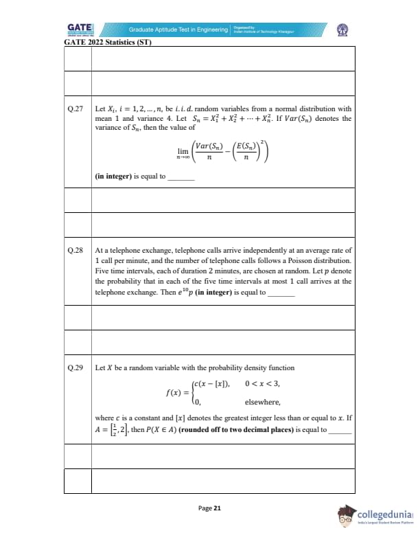
Let \( X_i, i = 1, 2, \dots, n \), be i.i.d. random variables from a normal distribution with mean 1 and variance 4. Let \( S_n = X_1^2 + X_2^2 + \dots + X_n^2 \). If \( Var(S_n) \) denotes the variance of \( S_n \), then the value of

(in integer) is equal to ________.
At a telephone exchange, telephone calls arrive independently at an average rate of 1 call per minute, and the number of telephone calls follows a Poisson distribution. Five time intervals, each of duration 2 minutes, are chosen at random. Let \( p \) denote the probability that in each of the five time intervals at most 1 call arrives at the telephone exchange. Then \( e^{10} p \) (in integer) is equal to ________
Let \( X \) be a random variable with the probability density function \[ f(x) = \begin{cases} c(x - \lfloor x \rfloor), & 0 < x < 3,
0, & elsewhere, \end{cases} \]
where \( c \) is a constant and \( \lfloor x \rfloor \) denotes the greatest integer less than or equal to \( x \). If A = [1/2,2] then P(X ∈ A) (rounded off to two decimal places) is equal to ________.
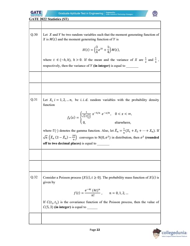
Let \( X \) and \( Y \) be two random variables such that the moment generating function of \( X \) is \( M(t) \) and the moment generating function of \( Y \) is \[ H(t) = \left( \frac{3}{4} e^{2t} + \frac{1}{4} \right) M(t), \]
where \( t \in (-h, h), h > 0 \). If the mean and the variance of \( X \) are \( \frac{1}{2} \) and \( \frac{1}{4} \), respectively, then the variance of \( Y \) (in integer) is equal to ________
Let \( X_i, i = 1, 2, \dots, n \), be i.i.d. random variables with the probability density function \[ f_X(x) = \begin{cases} \frac{1}{\sqrt{2 \Gamma\left( \frac{1}{6} \right)}} x^{-\frac{5}{6}} e^{-\frac{x}{8}}, & 0 < x < \infty,
0, & elsewhere, \end{cases} \]
where \( \Gamma(\cdot) \) denotes the gamma function. Also, let \( \bar{X}_n = \frac{1}{n} (X_1 + X_2 + \cdots + X_n) \). If \[ \sqrt{n} \left( \bar{X}_n - \mathbb{E}[\bar{X}_n] \right) \xrightarrow{d} N(0, \sigma^2), \]
then \( \sigma^2 \) (rounded off to two decimal places) is equal to ________
Consider a Poisson process \( \{ X(t), t \geq 0 \} \). The probability mass function of \( X(t) \) is given by \[ f(t) = \frac{e^{-4t} (4t)^n}{n!}, \quad n = 0, 1, 2, \dots \]
If \( C(t_1, t_2) \) is the covariance function of the Poisson process, then the value of C(5, 3) (in integer) is equal to ________.
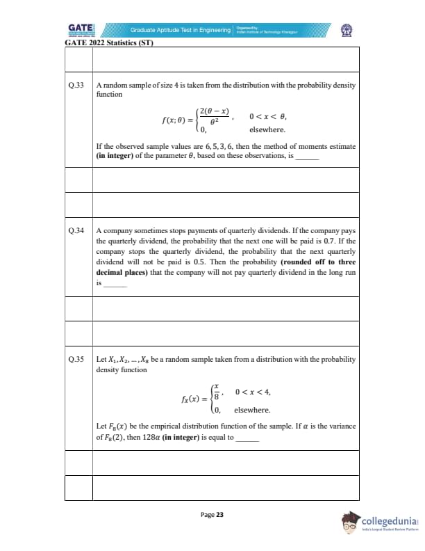
A random sample of size 4 is taken from the distribution with the probability density function \[ f(x; \theta) = \begin{cases} \frac{2(\theta - x)}{\theta^2}, & 0 < x < \theta,
0, & elsewhere. \end{cases} \]
If the observed sample values are 6, 5, 3, 6, then the method of moments estimate (in integer) of the parameter \( \theta \), based on these observations, is ________
A company sometimes stops payments of quarterly dividends. If the company pays the quarterly dividend, the probability that the next one will be paid is 0.7. If the company stops the quarterly dividend, the probability that the next quarterly dividend will not be paid is 0.5. Then the probability (rounded off to three decimal places) that the company will not pay quarterly dividend in the long run is ________
Let \( X_1, X_2, \dots, X_8 \) be a random sample taken from a distribution with the probability density function \[ f_X(x) = \begin{cases} \frac{x}{8}, & 0 < x < 4,
0, & elsewhere. \end{cases} \]
Let \( F_8(x) \) be the empirical distribution function of the sample. If \( \alpha \) is the variance of \( F_8(2) \), then 128\( \alpha \) (in integer) is equal to ________
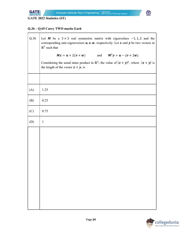
Let \( M \) be a 3 \(\times\) 3 real symmetric matrix with eigenvalues \(-1, 1, 2\) and the corresponding unit eigenvectors \( u, v, w \), respectively. Let \( x \) and \( y \) be two vectors in \( \mathbb{R}^3 \) such that \[ Mx = u + 2(v + w) \quad and \quad M^2 y = u - (v + 2w). \]
Considering the usual inner product in \( \mathbb{R}^3 \), the value of \( |x + y|^2 \), where \( |x + y| \) is the length of the vector \( x + y \), is
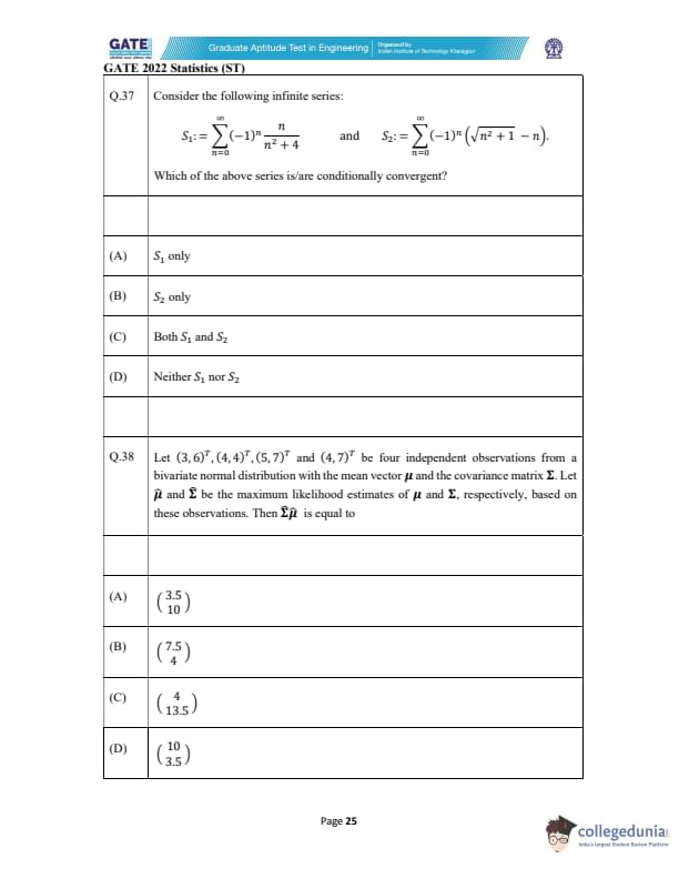
Consider the following infinite series: \[ S_1 := \sum_{n=0}^{\infty} (-1)^n \frac{n}{n^2 + 4} \quad and \quad S_2 := \sum_{n=0}^{\infty} (-1)^n \sqrt{n^2 + 1 - n}. \]
Which of the above series is/are conditionally convergent?
Let \( (3, 6)^T, (4, 4)^T, (5, 7)^T \) and \( (4, 7)^T \) be four independent observations from a bivariate normal distribution with the mean vector \( \mu \) and the covariance matrix \( \Sigma \). Let \( \hat{\mu} \) and \( \hat{\Sigma} \) be the maximum likelihood estimates of \( \mu \) and \( \Sigma \), respectively, based on these observations. Then \( \hat{\Sigma} \hat{\mu} \) is equal to

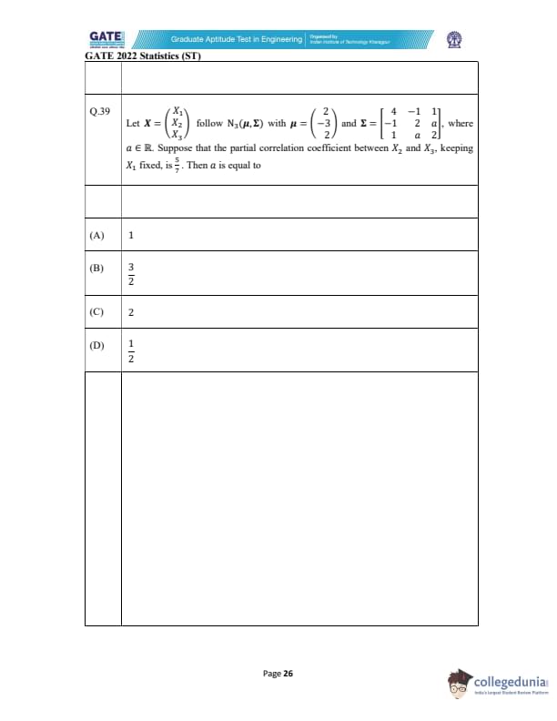
Let \( X = \begin{pmatrix} X_1
X_2
X_3 \end{pmatrix} \) follow \( N_3(\mu, \Sigma) \) with \( \mu = \begin{pmatrix} 2
-3
2 \end{pmatrix} \) and \( \Sigma = \begin{pmatrix} 4 & -1 & 1
-1 & 2 & a
1 & a & 2 \end{pmatrix} \), where \( a \in \mathbb{R} \). Suppose that the partial correlation coefficient between \( X_2 \) and \( X_3 \), keeping \( X_1 \) fixed, is \( \frac{5}{7} \). Then \( a \) is equal to
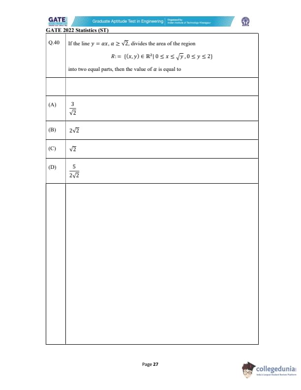
If the line \( y = \alpha x, \alpha \geq \sqrt{2} \), divides the area of the region \[ R := \{(x, y) \in \mathbb{R}^2 \mid 0 \leq x \leq \sqrt{y}, 0 \leq y \leq 2\} \]
into two equal parts, then the value of \( \alpha \) is equal to
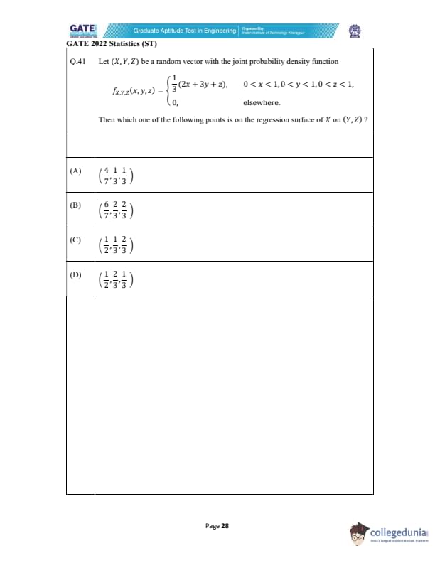
Let \( (X, Y, Z) \) be a random vector with the joint probability density function \[ f_{X,Y,Z}(x, y, z) = \begin{cases} \frac{1}{3}(2x + 3y + z), & 0 < x < 1, 0 < y < 1, 0 < z < 1,
0, & elsewhere. \end{cases} \]
Then which one of the following points is on the regression surface of \( X \) on \( (Y, Z) \)?
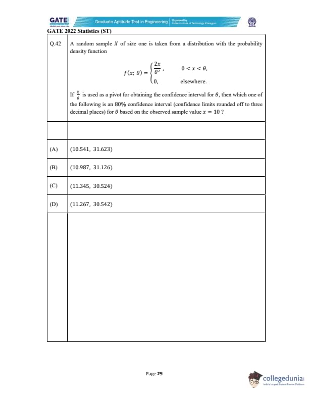
A random sample \( X \) of size one is taken from a distribution with the probability density function \[ f(x; \theta) = \begin{cases} \frac{2x}{\theta^2}, & 0 < x < \theta,
0, & elsewhere. \end{cases} \]
If \( \frac{X}{\theta} \) is used as a pivot for obtaining the confidence interval for \( \theta \), then which one of the following is an 80% confidence interval (confidence limits rounded off to three decimal places) for \( \theta \) based on the observed sample value \( x = 10 \)?
Let \( X_1, X_2, \dots, X_7 \) be a random sample from a normal population with mean 0 and variance \( \theta > 0 \). Let \[ K = \frac{X_1^2 + X_2^2 + \dots + X_7^2}{X_1^2 + X_2^2 + \dots + X_7^2}. \]
Consider the following statements:
The statistics \( K \) and \( X_1^2 + X_2^2 + \dots + X_7^2 \) are independent.
\( \frac{7K}{2} \) has an \( F \)-distribution with 2 and 7 degrees of freedom.
\( E(K^2) = \frac{8}{63} \).
Then which of the above statements is/are true?
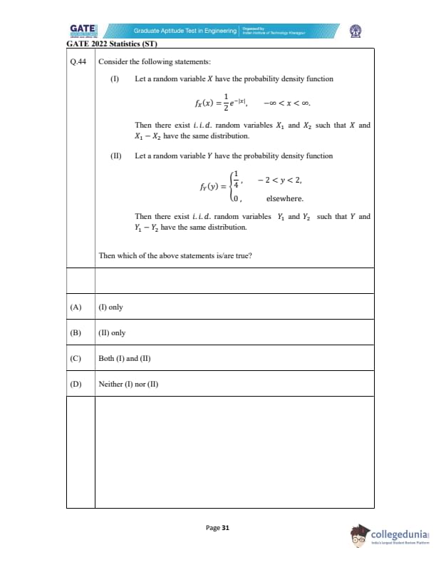
Consider the following statements:
(I) Let a random variable \(X\) have the probability density function \[ f_X(x) = \frac{1}{2} e^{-|x|}, \quad -\infty < x < \infty. \]
Then there exist i.i.d. random variables \(X_1\) and \(X_2\) such that \(X\) and \(X_1 - X_2\) have the same distribution.
(II) Let a random variable \(Y\) have the probability density function \[ f_Y(y) = \begin{cases} \frac{1}{4}, & -2 < y < 2,
0, & elsewhere. \end{cases} \]
Then there exist i.i.d. random variables \(Y_1\) and \(Y_2\) such that \(Y\) and \(Y_1 - Y_2\) have the same distribution.
Then which of the above statements is/are true?
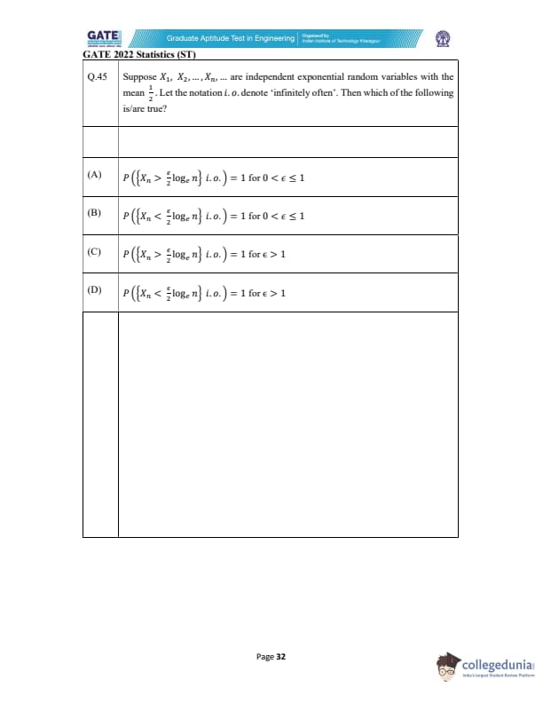
Suppose \( X_1, X_2, \dots, X_n, \dots \) are independent exponential random variables with the mean \( \frac{1}{2} \). Let the notation \( i.o. \) denote "infinitely often." Then which of the following is/are true?
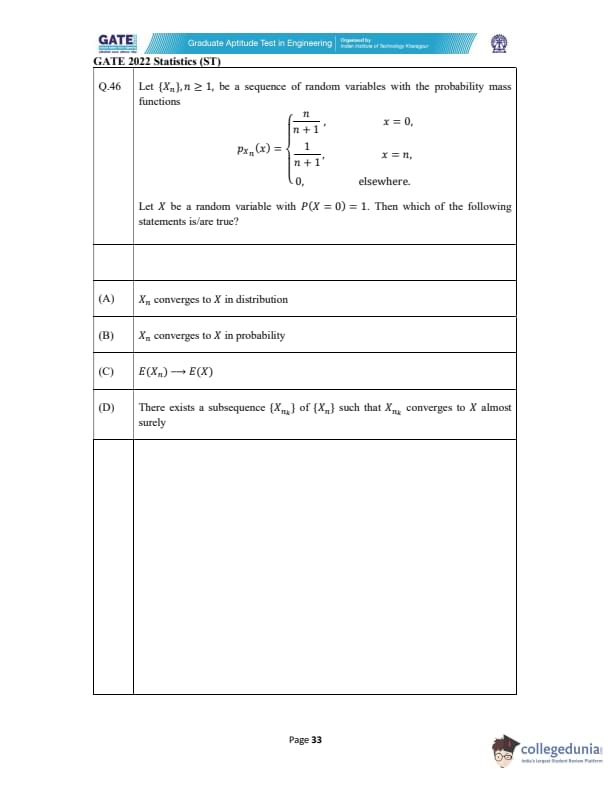
Let \( \{ X_n \}, n \geq 1 \), be a sequence of random variables with the probability mass functions \[ p_{X_n}(x) = \begin{cases} \frac{n}{n+1}, & x = 0
\frac{1}{n+1}, & x = n
0, & elsewhere \end{cases} \]
Let \( X \) be a random variable with \( P(X = 0) = 1 \). Then which of the following statements is/are true?
Let \(M\) be any \(3\times3\) symmetric matrix with eigenvalues \(1,2,3\). Let \(N\) be any \(3\times3\) matrix with real eigenvalues such that \(MN+N^{T}M=3I\), where \(I\) is the \(3\times3\) identity matrix. Which of the following cannot be eigenvalue(s) of the matrix \(N\)?
Let \( M \) be a \( 3 \times 2 \) real matrix having a singular value decomposition as \( M = U S V^T \), where the matrix \( S = \begin{bmatrix} \sqrt{3} & 0
0 & 1
0 & 0 \end{bmatrix}^T \), \( U \) is a \( 3 \times 3 \) orthogonal matrix, and \( V \) is a \( 2 \times 2 \) orthogonal matrix. Then which of the following statements is/are true?
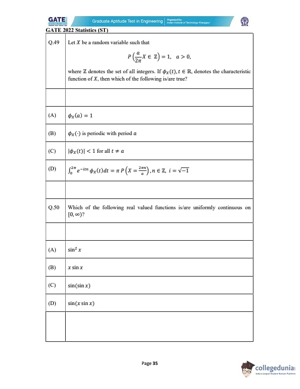
Let \( X \) be a random variable such that \[ P \left( \frac{a}{2\pi} X \in \mathbb{Z} \right) = 1, \quad a > 0, \]
where \( \mathbb{Z} \) denotes the set of all integers. If \( \phi_X(t), t \in \mathbb{R} \), denotes the characteristic function of \( X \), then which of the following is/are true?
Which of the following real-valued functions is/are uniformly continuous on \([0, \infty)\)?
Two independent random samples, each of size 7, from two populations yield the following values:

If Mann–Whitney \( U \) test is performed at 5% level of significance to test the null hypothesis \( H_0: \) Distributions of the populations are same, against the alternative hypothesis \( H_1: \) Distributions of the populations are not same, then the value of the test statistic \( U \) (in integer) for the given data, is ________
Consider the multiple regression model \[ Y = \beta_0 + \beta_1 X_1 + \beta_2 X_2 + \beta_3 X_3 + \epsilon, \]
where \( \epsilon \) is normally distributed with mean 0 and variance \( \sigma^2 > 0 \), and \( \beta_0, \beta_1, \beta_2, \beta_3 \) are unknown parameters. Suppose 52 observations of \( (Y, X_1, X_2, X_3) \) yield sum of squares due to regression as 18.6 and total sum of squares as 79.23. Then, for testing the null hypothesis \( H_0: \beta_1 = \beta_2 = \beta_3 = 0 \) against the alternative hypothesis \( H_1: \beta_i \neq 0 \) for some \( i = 1, 2, 3 \), the value of the test statistic (rounded off to three decimal places), based on one way analysis of variance, is ________
Suppose a random sample of size 3 is taken from a distribution with the probability density function \[ f(x) = \begin{cases} 2x, & 0 < x < 1,
0, & elsewhere. \end{cases} \]
If \( p \) is the probability that the largest sample observation is at least twice the smallest sample observation, then the value of \( p \) (rounded off to three decimal places) is ________
Let a linear model \( Y = \beta_0 + \beta_1 X + \epsilon \) be fitted to the following data, where \( \epsilon \) is normally distributed with mean 0 and unknown variance \( \sigma^2 > 0 \):

Let \( \hat{Y}_0 \) denote the ordinary least-square estimator of \( Y \) at \( X = 6 \), and the variance of \( \hat{Y}_0 \) be \( c\sigma^2 \). Then the value of the real constant \( c \) (rounded off to one decimal place) is equal to ________
Let \(0,1,1,2,0\) be five observations of a random variable \(X\) which follows a Poisson distribution with parameter \(\theta>0\). Let the minimum variance unbiased estimate of \(P(X\le 1)\), based on this data, be \(\alpha\). Then \(5^{4}\alpha\) (in integer) is equal to \(\;\_\_\_\_\_\)
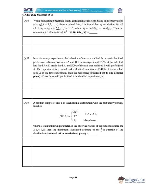
While calculating Spearman’s rank correlation coefficient on \(n\) paired observations, it is found that \(x_i\) are distinct for all \(i\ge 2\), with a single tie \(x_1=x_2\), and \(\sum_{i=1}^{n} d_i^2=19.5\) where \(d_i=rank(x_i)-rank(y_i)\). Then the minimum possible value of \(\,n^3-n\,\) (in integer) is \(\;\_\_\_\_\_\).
In a laboratory experiment, cats choose between foods A and B. If a cat had A, it will prefer A next time with probability \(0.7\); if it had B, it will prefer A next time with probability \(0.5\). The experiment is repeated under identical conditions. If \(40%\) cats had A in the first experiment, then the percentage (rounded off to one decimal place) of cats that will prefer A in the third experiment is _____.
A random sample of size \(5\) is taken from the distribution with density function

where \(\theta\) is unknown. If the observations are \(3,6,4,7,5\), then the maximum likelihood estimate of the \(1/8\) quantile of the distribution (rounded off to one decimal place) is _____.
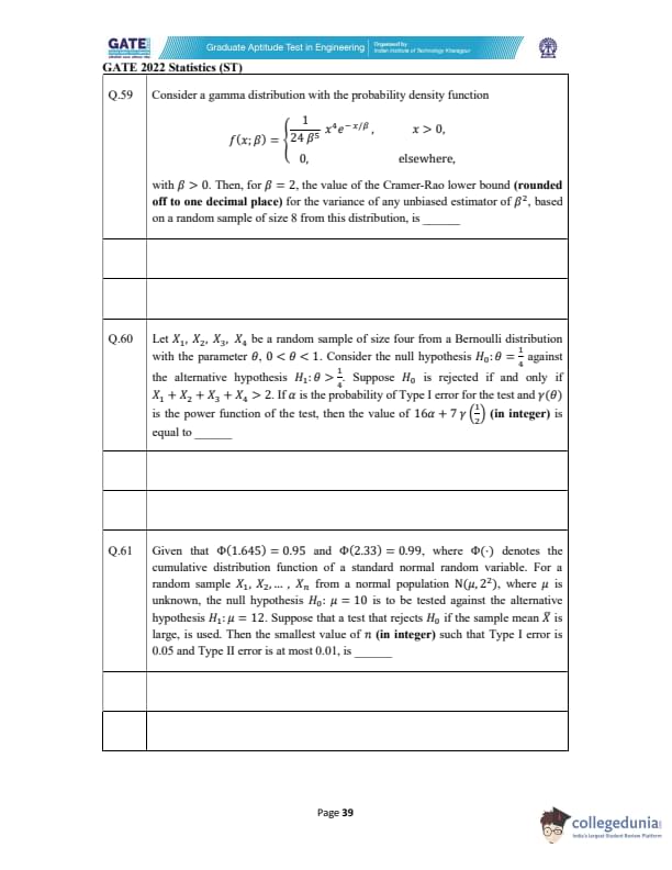
Consider a gamma distribution with pdf \[ f(x;\beta)= \begin{cases} \dfrac{1}{24\beta^{5}}x^{4}e^{-x/\beta}, & x>0,
0, & elsewhere, \end{cases} \]
with \(\beta>0\). For \(\beta=2\), find the Cramér–Rao lower bound (rounded to one decimal place) for the variance of any unbiased estimator of \(\beta^{2}\) based on a random sample of size 8.
Let \(X_1,X_2,X_3,X_4\) be a sample of size 4 from Bernoulli(\(\theta\)), \(0<\theta<1\).
We test \(H_0:\theta=\tfrac14\) vs \(H_1:\theta>\tfrac14\), rejecting \(H_0\) if \(X_1+X_2+X_3+X_4>2\).
If \(\alpha\) is the Type-I error and \(\gamma(\theta)\) the power function, then find \(16\alpha+7\gamma\!\left(\tfrac12\right)\) (in integer).
Given \(\Phi(1.645)=0.95\) and \(\Phi(2.33)=0.99\). For a random sample \(X_1,\ldots,X_n\sim N(\mu,2^2)\) with \(\mu\) unknown, test \(H_0:\mu=10\) vs \(H_1:\mu=12\) using a rule that rejects \(H_0\) when \(\overline X\) is large. Find the smallest \(n\) (in integer) so that Type I error is \(0.05\) and Type II error is at most \(0.01\).
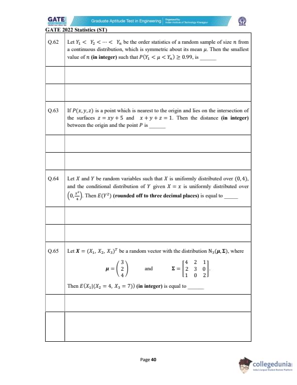
Let Y1< Y2< ……...< Yn be order statistics from a continuous distribution symmetric about its mean $\mu$. Find the smallest n (in integer) such that P(Y1 < \mu < Yn)≥ 0.99.
If \(P(x,y,z)\) is the point nearest to the origin lying on the intersection of the surfaces \(z=xy+5\) and \(x+y+z=1\), then the distance (in integer) between the origin and \(P\) is _____.
Let \(X\sim Unif(0,4)\) and, given \(X=x\), \(Y\mid X=x\sim Unif\!\left(0,\dfrac{x^{2}}{4}\right)\). Compute \(E(Y^{2})\) (rounded off to three decimal places).
Let \(X=(X_1,X_2,X_3)^{T}\sim N_3(\mu,\Sigma)\) where \[ \mu=\begin{pmatrix}3
2
4\end{pmatrix},\qquad \Sigma=\begin{pmatrix} 4 & 2 & 1
2 & 3 & 0
1 & 0 & 2 \end{pmatrix}. \]
Find \(E[X_1\mid(X_2=4,X_3=7)]\) (in integer).


Quick Links:
GATE 2022 ST Detailed Paper Analysis
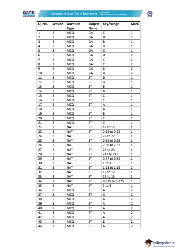
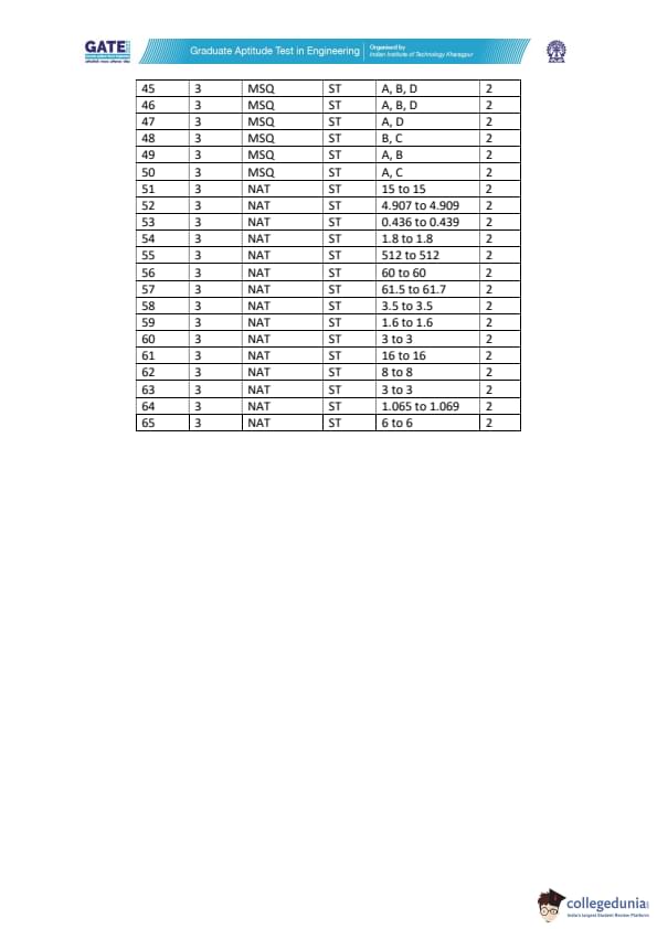
IIT Kharagpur listed MCQs (Multiple Choice Questions), MSQs (Multiple Select Questions), NATs (Numerical Answer Type) questions to constitute the question paper of GATE 2022 ST. Have a look at the below-mentioned table in order to get details of questions as per the carried marks-
| Question Types | Question Frequency | Carried Marks |
|---|---|---|
| No. Of 1 mark MCQs | 16 | 16 |
| No. Of 2 mark MCQs | 14 | 28 |
| No. Of 1 mark MSQs | - | - |
| No. Of 2 marks MSQs | 6 | 12 |
| No. Of 1 mark NATs | 14 | 14 |
| No. Of 2 marks NATs | 15 | 30 |
| Total | 65 | 100 |
- The General Aptitude section was accountable for carrying 10 questions. The rest of the 55 questions were carried by core Statistics based topics
- MSQs carried the least weightage in exam
- Equal weightage was carried by MCQs and NATs
Also Check:
GATE 2022 ST: Exam Pattern and Marking Scheme
- GATE 2022 ST asked both MCQs and NATs. It was held online via CBT mode
- As per the specified marking scheme by IIT Delhi, from the final score, ⅓ and ⅔ marks would be reduced for each wrong MCQ carried 1 and 2 marks
- Wrong attempted NATs were not supposed to bring any kind of deduction in the final achieved marks
GATE Previous Year Question Papers
| GATE 2022 Question Papers | GATE 2021 Question Papers | GATE 2020 Question Papers |
| GATE 2019 Question Papers | GATE 2018 Question Papers | GATE 2017 Question Papers |


Comments