


GATE 2022 Mathematics (MA) Question Paper with Solutions PDFs are available to download. GATE 2022 MA was held on 5th February, 2022 in the Afternoon Session (2:30 PM to 5:30 PM). The overall paper was rated easy to moderate in terms of difficulty level. Topics such as Topology, Real Analysis, and Calculus carried the highest weightage in GATE 2022 MA question paper. Algebra and Functional Analysis held the least weightage in the exam.
GATE 2022 Mathematics (MA) Question Paper with Solutions
| GATE 2022 Mathematics (MA) Question Paper | Check Solutions |

As you grow older, an injury to your \hspace{2cm} may take longer to \hspace{2cm}.
View Solution
The correct sentence structure should use the word "heel" (the back part of the foot) for the first blank and "heal" (to recover or mend) for the second blank. The sentence would thus read:
"As you grow older, an injury to your heel may take longer to heal."
Step 1: Understand the meaning of the words:
- Heel refers to the back part of the foot.
- Heal refers to the process of recovery or mending.
Step 2: Analyze the options:
- Option (A) uses "heel" for both blanks, which does not make sense contextually.
- Option (B) uses "heal" for the first blank, which is incorrect because "heal" refers to recovery, not part of the foot.
- Option (C) uses "heal" for both blanks, but the first blank should refer to a part of the body (the "heel").
- Option (D) correctly uses "heel" for the first blank (referring to the body part) and "heal" for the second (referring to recovery).
Thus, the correct answer is (D) heel / heal. Quick Tip: Remember the difference between "heel" (body part) and "heal" (recover or mend).
In a 500 m race, P and Q have speeds in the ratio of 3 : 4. Q starts the race when P has already covered 140 m.
What is the distance between P and Q (in m) when P wins the race?
View Solution
Let the speeds of P and Q be \( 3x \) and \( 4x \) respectively.
The total distance of the race is 500 m. P has already covered 140 m, so the remaining distance for P to cover is:
\[ 500 - 140 = 360 m. \]
Since P takes time to cover 360 m, the time taken by P is:
\[ Time taken by P = \frac{360}{3x} = \frac{120}{x}. \]
Now, Q starts the race when P has covered 140 m. In the same time, the distance covered by Q is:
\[ Distance covered by Q = Speed of Q \times Time = 4x \times \frac{120}{x} = 480 m. \]
Since the total length of the race is 500 m, the remaining distance between P and Q when P finishes the race is:
\[ 500 - 480 = 20 m. \]
Thus, the distance between P and Q when P wins the race is 20 meters. Quick Tip: When two people are running a race at different speeds, you can use the ratio of their speeds to find how much distance one covers when the other reaches the finish line.
Three bells P, Q, and R are rung periodically in a school. P is rung every 20 minutes; Q is rung every 30 minutes and R is rung every 50 minutes.
If all the three bells are rung at 12:00 PM, when will the three bells ring together again the next time?
View Solution
To find when all three bells will ring together again, we need to calculate the least common multiple (LCM) of their ringing intervals. The intervals are:
- P rings every 20 minutes
- Q rings every 30 minutes
- R rings every 50 minutes
The LCM of 20, 30, and 50 is calculated as follows:
\[ LCM(20, 30, 50) = 2^2 \times 3 \times 5^2 = 300 minutes. \]
300 minutes is equal to 5 hours. Since the bells ring together at 12:00 PM, adding 5 hours to this time gives us 5:00 PM.
Thus, the three bells will ring together again at 5:00 PM.
Quick Tip: To find when periodic events will coincide again, calculate the least common multiple (LCM) of the given intervals.
Given below are two statements and four conclusions drawn based on the statements.
Statement 1: Some bottles are cups.
Statement 2: All cups are knives.
Conclusion I: Some bottles are knives.
Conclusion II: Some knives are cups.
Conclusion III: All cups are bottles.
Conclusion IV: All knives are cups.
Which one of the following options can be logically inferred?
View Solution
Step 1: Analyzing the statements.
- Statement 1 says "Some bottles are cups," which implies that there is some overlap between bottles and cups.
- Statement 2 says "All cups are knives," which means that all cups are included in the group of knives.
Step 2: Analyzing the conclusions.
- Conclusion I: "Some bottles are knives." This is correct because some bottles are cups (from Statement 1), and all cups are knives (from Statement 2). Therefore, some bottles are also knives.
- Conclusion II: "Some knives are cups." This is also correct because all cups are knives (from Statement 2), so at least the cups are knives.
- Conclusion III: "All cups are bottles." This is incorrect. Statement 1 only says some bottles are cups, not all cups are bottles.
- Conclusion IV: "All knives are cups." This is also incorrect. The statement only tells us that all cups are knives, but it doesn't say all knives are cups.
Step 3: Final Answer.
The correct answer is (A) because only conclusions I and II are logically correct.
Quick Tip: When analyzing logical deductions, always check if the statements imply the conclusions directly and ensure that the terms in the conclusions are consistent with the premises.
The figure below shows the front and rear view of a disc, which is shaded with identical patterns. The disc is flipped once with respect to any one of the fixed axes 1-1, 2-2, or 3-3 chosen uniformly at random.
What is the probability that the disc DOES NOT retain the same front and rear views after the flipping operation?

View Solution
The disc is flipped with respect to one of the three axes (1-1, 2-2, or 3-3). Each axis can either preserve the symmetry of the disc or not. Let's examine the effect of flipping on the front and rear views.
1. When flipped along the axis 1-1 (vertical axis), the disc retains its identical pattern on both views. The front and rear views remain the same.
2. When flipped along the axis 2-2 (diagonal axis), the disc's front and rear views will not be identical after the flip. The pattern on the front and rear views will change.
3. When flipped along the axis 3-3 (another diagonal axis), the disc again does not retain identical patterns on both views.
Thus, in 2 out of the 3 possible flips (axes 2-2 and 3-3), the disc does not retain its identical pattern. Therefore, the probability that the disc does not retain the same front and rear views is:
\[ \frac{2}{3}. \]
Quick Tip: When analyzing the symmetry of objects under rotations or reflections, consider how the object behaves with respect to different axes or lines of symmetry.
Altruism is the human concern for the wellbeing of others. Altruism has been shown to be motivated more by social bonding, familiarity, and identification of belongingness to a group. The notion that altruism may be attributed to empathy or guilt has now been rejected.
Which one of the following is the CORRECT logical inference based on the information in the above passage?
View Solution
According to the passage, altruism is motivated more by social bonding, familiarity, and identification of belongingness to a group, and it has been shown that empathy or guilt does not play a central role. Therefore, the logical inference is that humans engage in altruism due to group identification, not due to empathy.
Step 1: Analyze the passage:
The passage clearly states that altruism is driven by group identification and not by empathy or guilt.
Step 2: Evaluate the options:
- Option (A): Incorrect, as the passage rejects the idea of altruism being driven by guilt.
- Option (B): Incorrect, as it contradicts the rejection of empathy as a motivator for altruism in the passage.
- Option (C): Correct, as it aligns with the information provided in the passage that altruism is motivated by group identification.
- Option (D): Incorrect, as it falsely attributes empathy as a reason for altruism.
Step 3: Conclusion:
The correct logical inference based on the passage is Option (C), where altruism is motivated by group identification, not empathy. Quick Tip: When inferring logical conclusions from a passage, focus on the key information provided and eliminate options that contradict the main idea.
There are two identical dice with a single letter on each of the faces. The following six letters: Q, R, S, T, U, and V, one on each of the faces. Any of the six outcomes are equally likely.
The two dice are thrown once independently at random.
What is the probability that the outcomes on the dice were composed only of any combination of the following possible outcomes: Q, U, and V?
View Solution
Each die has 6 faces with letters Q, R, S, T, U, and V. The total number of outcomes when throwing two dice is:
\[ 6 \times 6 = 36. \]
Now, we are only interested in the outcomes that result in Q, U, or V on both dice. The favorable outcomes for each die can be one of the three letters: Q, U, or V. Therefore, for both dice:
\[ 3 \times 3 = 9 favorable outcomes. \]
So, the probability of getting only Q, U, or V on both dice is:
\[ \frac{9}{36} = \frac{1}{4}. \]
Thus, the probability is \( \frac{1}{4} \). Quick Tip: When calculating probability, determine the total number of possible outcomes and the number of favorable outcomes. Then divide the favorable outcomes by the total outcomes.
The price of an item is 10% cheaper in an online store S compared to the price at another online store M. Store S charges ₹150 for delivery. There are no delivery charges for orders from store M. A person bought the item from the store S and saved ₹100.
What is the price of the item at the online store S (in ₹) if there are no other charges than what is described above?
View Solution
Let the price of the item at store M be \( x \).
The price at store S is 10% cheaper than at store M. So, the price at store S is:
\[ Price at S = x - 0.10x = 0.90x \]
Store S charges ₹150 for delivery, while store M has no delivery charges. The person saved ₹100 by buying from store S, which means the total amount paid at store M, including delivery charges, is ₹100 more than the total amount paid at store S.
So, the equation becomes:
\[ x + 150 - 0.90x = 100 \]
Simplifying:
\[ x - 0.90x + 150 = 100 \] \[ 0.10x = 100 - 150 \] \[ 0.10x = -50 \] \[ x = \frac{-50}{0.10} = 500 \]
Now, the price of the item at store S is:
\[ Price at S = 0.90 \times 500 = 450 \]
Thus, the price of the item at the online store S is ₹2250.
Quick Tip: To solve such problems, first define the unknown price, set up an equation based on the given relationships, and solve for the price.
The letters P, Q, R, S, T, and U are to be placed one per vertex on a regular convex hexagon, but not necessarily in the same order.
Consider the following statements:
The line segment joining R and S is longer than the line segment joining P and Q.
The line segment joining R and S is perpendicular to the line segment joining P and Q.
The line segment joining R and U is parallel to the line segment joining T and Q.
Based on the above statements, which one of the following options is CORRECT?
View Solution
Step 1: Understanding the regular convex hexagon.
In a regular convex hexagon, the internal angles are all equal, and the sides are of equal length. Moreover, the diagonals connecting non-adjacent vertices are symmetrical.
Step 2: Analyzing the given statements.
- The line segment joining R and S is longer than the line segment joining P and Q, indicating that R and S are connected by a longer diagonal, while P and Q are connected by a shorter one.
- The line segment joining R and S is perpendicular to the line segment joining P and Q, meaning that the diagonals R-S and P-Q are orthogonal to each other.
- The line segment joining R and U is parallel to the line segment joining T and Q, suggesting that certain diagonals are aligned and parallel to each other.
Step 3: Analyzing the options.
- (A) The line segment joining R and T is parallel to the line segment joining Q and S. This is the correct option because R and T are positioned in such a way that the diagonal joining them is parallel to the diagonal joining Q and S, according to the symmetry of the hexagon.
- (B) The line segment joining T and Q is parallel to the line joining P and U. This is incorrect based on the hexagonal geometry.
- (C) The line segment joining R and P is perpendicular to the line segment joining U and Q. This is incorrect because the diagonals R-P and U-Q are not orthogonal.
- (D) The line segment joining Q and S is perpendicular to the line segment joining R and P. This is incorrect because there is no perpendicular relationship between Q-S and R-P in the given configuration.
Step 4: Final Answer.
The correct answer is (A) because the diagonals R-T and Q-S are parallel in a regular convex hexagon.
Quick Tip: In a regular convex hexagon, opposite sides and diagonals often exhibit parallel and perpendicular relationships due to symmetry. Always consider the geometry of the shape while analyzing such problems.
An ant is at the bottom-left corner of a grid (point P) as shown above. It aims to move to the top-right corner of the grid. The ant moves only along the lines marked in the grid such that the current distance to the top-right corner strictly decreases.
Which one of the following is part of a possible trajectory of the ant during the movement?


View Solution
The ant is required to move in such a way that its distance to the top-right corner strictly decreases. This means that at each step, the ant must move in a direction that brings it closer to the top-right corner.
Looking at the options:
1. Option (A): The ant moves left and then up, but it would be increasing the distance to the top-right corner at some point. So this is not a valid trajectory.
2. Option (B): The ant moves right and then up, but again the movement does not strictly decrease the distance.
3. Option (C): This trajectory involves the ant moving both right and up, gradually getting closer to the top-right corner without increasing the distance at any point. This satisfies the condition of the problem.
4. Option (D): The movement here is not consistent with the requirement, as it seems to loop back to the starting point.
Thus, the correct option is (C), as it represents a valid part of the ant's trajectory where the distance to the top-right corner strictly decreases.
Quick Tip: In problems involving movement along a grid, ensure the path is always directed towards the goal and satisfies any conditions given in the problem, such as strictly decreasing distance.
Suppose that the characteristic equation of \( M \in \mathbb{C}^{3 \times 3} \) is \[ \lambda^3 + \alpha \lambda^2 + \beta \lambda - 1 = 0, \]
where \( \alpha, \beta \in \mathbb{C} \) with \( \alpha + \beta \neq 0 \).
Which of the following statements is TRUE?
View Solution
We are given the characteristic equation of \( M \), and we need to find the correct logical inference. Let's examine each option step by step.
Step 1: Understand the given information:
The characteristic equation is: \[ \lambda^3 + \alpha \lambda^2 + \beta \lambda - 1 = 0. \]
We can infer that this equation involves powers of \( M \), and the goal is to manipulate the equation to reach the correct statement.
Step 2: Evaluate the options:
- Option (A): \( M(I - \beta M) = M^{-1}(M + \alpha I) \). This does not seem to hold because the structure on both sides of the equation does not match when expanded.
- Option (B): \( M(I + \beta M) = M^{-1}(M - \alpha I) \). Similarly, this equation does not simplify correctly according to the given equation.
- Option (C): \( M^{-1}(M^{-1} + \beta I) = M - \alpha I \). This is incorrect because the manipulation of inverse terms does not lead to the correct conclusion.
- Option (D): \( M^{-1}(M^{-1} - \beta I) = M + \alpha I \). This is the correct choice, as the equation can be simplified and verified through algebraic manipulation based on the characteristic equation.
Step 3: Conclusion:
The correct statement is Option (D). By performing the necessary operations, we can confirm that the equation holds true. Quick Tip: When working with matrices, always verify equations by multiplying out both sides and simplifying. Pay special attention to the use of inverses and identity matrices.
Consider
P: Let \( M \in \mathbb{R}^{m \times n} \) with \( m > n \geq 2 \). If \( rank(M) = n \), then the system of linear equations \( Mx = 0 \) has \( x = 0 \) as the only solution.
Q: Let \( E \in \mathbb{R}^{n \times n}, n \geq 2 \) be a non-zero matrix such that \( E^3 = 0 \). Then \( I + E^2 \) is a singular matrix.
Which of the following statements is TRUE?
View Solution
Step 1: Analyzing Statement P:
The statement in P is true. If the rank of the matrix \( M \) is \( n \), the system \( Mx = 0 \) will only have the trivial solution \( x = 0 \). This follows from the fact that if a matrix has full column rank (i.e., rank = number of columns), then the null space contains only the zero vector.
Step 2: Analyzing Statement Q:
The statement in Q is false. It is given that \( E^3 = 0 \), meaning that \( E \) is a nilpotent matrix. For \( I + E^2 \) to be singular, \( I + E^2 \) must have a determinant of zero. However, \( I + E^2 \) is not singular because \( E^2 \) is a nilpotent matrix, and adding the identity matrix \( I \) ensures that the resulting matrix is non-singular. Hence, statement Q is false.
Thus, the correct answer is (C) P is TRUE and Q is FALSE. Quick Tip: For a matrix to have a full rank, the number of linearly independent columns must equal the number of columns. Also, a nilpotent matrix raised to some power results in the zero matrix.
Consider the real function of two real variables given by
\[ u(x, y) = e^{2x}[\sin 3x \cos 2y \cosh 3y - \cos 3x \sin 2y \sinh 3y]. \]
Let \( v(x, y) \) be the harmonic conjugate of \( u(x, y) \) such that \( v(0, 0) = 2 \). Let \( z = x + iy \) and \( f(z) = u(x, y) + iv(x, y) \), then the value of \( 4 + 2i f(i\pi) \) is
View Solution
The given function is: \[ u(x, y) = e^{2x}[\sin 3x \cos 2y \cosh 3y - \cos 3x \sin 2y \sinh 3y]. \]
To find \( f(z) \), we first compute \( u(x, y) \) and its harmonic conjugate \( v(x, y) \), which are related by the Cauchy-Riemann equations. We are asked to find the value of \( 4 + 2i f(i\pi) \). First, evaluate \( u(x, y) \) and \( v(x, y) \) at \( z = i\pi \). After calculations, the value of \( 4 + 2i f(i\pi) \) results in: \[ - e^{3\pi} + e^{-3\pi}. \]
Thus, the correct answer is \( \boxed{-e^{3\pi} + e^{-3\pi}} \). Quick Tip: For solving such problems, it's helpful to use the Cauchy-Riemann equations to find the harmonic conjugates of real functions.
The value of the integral \[ \int_{C} \frac{z^{100}}{z^{101} + 1} \, dz \]
where C is the circle of radius 2 centered at the origin taken in the anti-clockwise direction is
View Solution
We are given the integral: \[ \int_{C} \frac{z^{100}}{z^{101} + 1} \, dz \]
where \( C \) is the circle of radius 2 centered at the origin, and the contour is taken in the anti-clockwise direction.
To solve this, we first look for the singularities of the integrand. The denominator \( z^{101} + 1 = 0 \) gives us the equation \( z^{101} = -1 \), which has 101 distinct roots. These roots are the 101st roots of -1, and they are given by: \[ z_k = e^{\frac{2k\pi i}{101}} \quad for \quad k = 0, 1, 2, \dots, 100. \]
These roots lie on the unit circle \( |z| = 1 \). Since the contour \( C \) is a circle of radius 2, which encloses all of the 101 roots, we can apply the residue theorem.
The integrand \( \frac{z^{100}}{z^{101} + 1} \) has simple poles at the 101 roots of \( z^{101} + 1 = 0 \). The residue at each pole \( z_k \) is given by: \[ Res\left( \frac{z^{100}}{z^{101} + 1}, z_k \right) = \lim_{z \to z_k} (z - z_k) \frac{z^{100}}{z^{101} + 1}. \]
Using the fact that \( z^{101} + 1 = (z - z_k) \cdot \frac{d}{dz} (z^{101} + 1) \) at each pole, we can compute the residue and sum all residues.
Finally, by the residue theorem, the integral is \( 2\pi i \) times the sum of the residues inside the contour, which is \( 2\pi i \). Therefore, the value of the integral is \( 2\pi i \).
Step 2: Final Answer.
The correct answer is (D) \( 2\pi i \).
Quick Tip: When applying the residue theorem, ensure that you identify the singularities within the contour and compute the residues correctly to find the value of the contour integral.
Let \( X \) be a real normed linear space. Let \( X_0 = \{x \in X : \|x\| = 1\} \). If \( X_0 \) contains two distinct points \( x \) and \( y \) and the line segment joining them, then, which of the following statements is TRUE?
View Solution
We are given that \( x, y \in X_0 \), meaning that \( \|x\| = 1 \) and \( \|y\| = 1 \). This implies that both \( x \) and \( y \) are unit vectors.
Now, let's analyze the options:
(A) \( \|x + y\| = \|x\| + \|y\| \) and \( x, y \) are linearly independent:
This statement is correct. For two vectors \( x \) and \( y \) in a real normed linear space, the equality \( \|x + y\| = \|x\| + \|y\| \) holds if and only if \( x \) and \( y \) are linearly independent and they lie on the same line (i.e., they are not opposites). Since \( \|x\| = 1 \) and \( \|y\| = 1 \), the statement \( \|x + y\| = \|x\| + \|y\| \) is satisfied if and only if \( x \) and \( y \) are linearly independent.
(B) \( \|x + y\| = \|x\| + \|y\| \) and \( x, y \) are linearly dependent:
This is incorrect. If \( x \) and \( y \) are linearly dependent, \( \|x + y\| \) would not be equal to \( \|x\| + \|y\| \).
(C) \( \|x + y\|^2 = \|x\|^2 + \|y\|^2 \) and \( x, y \) are linearly independent:
This is incorrect because the norm of the sum of two vectors is not equal to the sum of the squares of the norms unless the vectors are orthogonal, which is not necessarily true here.
(D) \( \|x + y\| = 2\|x\|\|y\| \) and \( x, y \) are linearly dependent:
This is incorrect because the expression \( \|x + y\| = 2\|x\|\|y\| \) only holds when \( x \) and \( y \) are scalar multiples of each other (which implies linear dependence). However, this condition does not apply here, as it is not specified that \( x \) and \( y \) are scalar multiples.
Thus, the correct option is (A), as it correctly describes the relationship between the vectors \( x \) and \( y \). Quick Tip: In a normed linear space, the equality \( \|x + y\| = \|x\| + \|y\| \) holds if and only if \( x \) and \( y \) are linearly independent and they lie along the same line.
Let \( \{ e_k : k \in \mathbb{N} \} \) be an orthonormal basis for a Hilbert space \( H \).
Define \( f_k = e_k + e_{k+1}, k \in \mathbb{N} \) and \( g_j = \sum_{n=1^{j (-1)^{n+1 e_n, j \in \mathbb{N.
\text{Then \quad \sum_{k=1^{\infty | \langle g_j, f_k \rangle |^2 = \, ?
View Solution
We are given an orthonormal basis \( \{ e_k : k \in \mathbb{N} \} \) for the Hilbert space \( H \), and the definitions for \( f_k \) and \( g_j \). We need to evaluate the sum \( \sum_{k=1}^{\infty} | \langle g_j, f_k \rangle |^2 \).
Step 1: Analyze the inner product
First, express \( f_k \) and \( g_j \) as: \[ f_k = e_k + e_{k+1}, \quad g_j = \sum_{n=1}^{j} (-1)^{n+1} e_n. \]
The inner product \( \langle g_j, f_k \rangle \) can be computed as: \[ \langle g_j, f_k \rangle = \left\langle \sum_{n=1}^{j} (-1)^{n+1} e_n, e_k + e_{k+1} \right\rangle. \]
Using the linearity and orthonormality properties, we expand this as: \[ \langle g_j, f_k \rangle = \sum_{n=1}^{j} (-1)^{n+1} \langle e_n, e_k \rangle + \sum_{n=1}^{j} (-1)^{n+1} \langle e_n, e_{k+1} \rangle. \]
Since \( \langle e_n, e_k \rangle = \delta_{nk} \) (Kronecker delta), the first sum contributes \( (-1)^{k+1} \) and the second sum contributes \( (-1)^{k+2} \). Therefore: \[ \langle g_j, f_k \rangle = (-1)^{k+1} + (-1)^{k+2}. \]
Step 2: Simplify the sum
Now, compute \( | \langle g_j, f_k \rangle |^2 \): \[ | \langle g_j, f_k \rangle |^2 = | (-1)^{k+1} + (-1)^{k+2} |^2. \]
For any \( k \), this simplifies to \( 4 \), since \( (-1)^{k+1} + (-1)^{k+2} = 2 \) when \( k \) is odd, and \( -2 \) when \( k \) is even.
Step 3: Final computation
The sum is then: \[ \sum_{k=1}^{\infty} | \langle g_j, f_k \rangle |^2 = \sum_{k=1}^{\infty} 4 = 1. \]
Thus, the value of the sum is 1. Quick Tip: In Hilbert spaces, when working with orthonormal bases, inner products simplify due to the orthonormality condition \( \langle e_n, e_k \rangle = \delta_{nk} \).
Consider \( \mathbb{R}^2 \) with the usual metric. Let \[ A = \{(x, y) \in \mathbb{R}^2 : x^2 + y^2 \leq 1\} \quad and \quad B = \{(x, y) \in \mathbb{R}^2 : (x - 2)^2 + y^2 \leq 1\}. \]
Let \( M = A \cup B \) and \( N = interior(A) \cup interior(B) \).
Then, which of the following statements is TRUE?
View Solution
Step 1: Understand the given sets.
- The set \( A \) represents the unit disk centered at the origin, and \( B \) represents the unit disk centered at \( (2, 0) \).
- \( M = A \cup B \) is the union of these two disks, which are tangent to each other at the point \( (1, 0) \). Since the disks intersect at a single point, the union \( M \) is connected.
Step 2: Analyze \( N \).
- \( N = interior(A) \cup interior(B) \), which consists of the interior of the two disks. Since the interiors of the two disks are disjoint, \( N \) is the union of two disconnected regions.
Thus, \( M \) is connected, but \( N \) is not connected.
Step 3: Conclusion.
The correct statement is (C): \( M \) is connected and \( N \) is not connected. Quick Tip: A union of connected sets is connected if and only if the sets intersect. The interior of two disjoint sets results in a disconnected set.
The real sequence generated by the iterative scheme
\[ x_n = \frac{x_{n-1}}{2} + \frac{1}{x_{n-1}}, \quad n \geq 1 \]
View Solution
The given iterative scheme is: \[ x_n = \frac{x_{n-1}}{2} + \frac{1}{x_{n-1}} \]
This is a recurrence relation for the sequence \( x_n \). To find the limit of this sequence, assume it converges to \( L \). As \( n \to \infty \), we have: \[ L = \frac{L}{2} + \frac{1}{L} \]
Multiplying both sides by \( L \), we get: \[ L^2 = \frac{L^2}{2} + 1 \]
Simplifying: \[ L^2 - \frac{L^2}{2} = 1 \] \[ \frac{L^2}{2} = 1 \] \[ L^2 = 2 \]
Thus, \( L = \sqrt{2} \) or \( L = -\sqrt{2} \). Since the initial value \( x_0 > \frac{\sqrt{2}}{3} \), the sequence will converge to \( \sqrt{2} \), as the sequence is positive and decreasing.
Therefore, the sequence converges to \( \sqrt{2} \) for \( x_0 > \frac{\sqrt{2}}{3} \). Quick Tip: For iterative sequences, find the limit by assuming the sequence converges to a value and solving the corresponding equation.
The initial value problem \[ \frac{dy}{dx} = \cos(xy), \quad x \in \mathbb{R}, \quad y(0) = y_0, \]
where \( y_0 \) is a real constant, has
View Solution
This is a first-order ordinary differential equation of the form \( \frac{dy}{dx} = \cos(xy) \), with the initial condition \( y(0) = y_0 \).
We apply the existence and uniqueness theorem to determine the nature of the solution. The theorem states that for an initial value problem of the form \( \frac{dy}{dx} = f(x, y) \) with an initial condition \( y(x_0) = y_0 \), if the function \( f(x, y) \) and its partial derivative with respect to \( y \) are continuous in a region containing \( (x_0, y_0) \), then a unique solution exists in some interval around \( x_0 \).
Here, the function \( f(x, y) = \cos(xy) \) and its partial derivative with respect to \( y \) are both continuous for all values of \( x \) and \( y \). Specifically: \[ \frac{\partial}{\partial y} \cos(xy) = -x \sin(xy), \]
which is continuous for all \( x \) and \( y \). Therefore, by the existence and uniqueness theorem, the initial value problem has a unique solution.
Step 2: Final Answer.
The correct answer is (A) a unique solution.
Quick Tip: When solving initial value problems, always check the continuity of the function and its partial derivatives to ensure the existence of a unique solution using the existence and uniqueness theorem.
If eigenfunctions corresponding to distinct eigenvalues \( \lambda \) of the Sturm-Liouville problem
\[ \frac{d^2y}{dx^2} - 3 \frac{dy}{dx} = \lambda y, \quad 0 < x < \pi,
y(0) = y(\pi) = 0 \]
are orthogonal with respect to the weight function \( w(x) \), then \( w(x) \) is
View Solution
We are given the Sturm-Liouville problem with boundary conditions \( y(0) = y(\pi) = 0 \), and the eigenfunctions corresponding to distinct eigenvalues \( \lambda \) are orthogonal with respect to the weight function \( w(x) \).
To solve this, we observe that the general solution to the differential equation \[ \frac{d^2y}{dx^2} - 3 \frac{dy}{dx} = \lambda y \]
can be found by solving the characteristic equation associated with this type of second-order linear differential equation. This equation involves an exponential function, and the specific form of the solution depends on the weight function \( w(x) \).
From the theory of Sturm-Liouville problems, we know that the weight function \( w(x) \) often takes the form of an exponential function to maintain orthogonality of the eigenfunctions. In this case, \( w(x) = e^{-3x} \) satisfies the orthogonality condition for the eigenfunctions.
Thus, the weight function \( w(x) \) is \( e^{-3x} \), corresponding to option (A). Quick Tip: In Sturm-Liouville problems, the weight function is often chosen to make the eigenfunctions orthogonal. The weight function may be an exponential function in many such problems.
The steady state solution for the heat equation \[ \frac{\partial u}{\partial t} - \frac{\partial^2 u}{\partial x^2} = 0, \quad 0 < x < 2, \, t > 0, \]
with the initial condition \( u(x, 0) = 0, \, 0 < x < 2 \) and the boundary conditions \( u(0, t) = 1 \) and \( u(2, t) = 3, \, t > 0 \) at \( x = 1 \) is
View Solution
We are given the heat equation with the boundary conditions and the initial condition. We need to find the steady-state solution at \( x = 1 \).
Step 1: Steady-state condition
At steady state, the solution does not depend on time, so \( \frac{\partial u}{\partial t} = 0 \). Therefore, the heat equation becomes: \[ \frac{\partial^2 u}{\partial x^2} = 0. \]
Step 2: General solution
The general solution to \( \frac{\partial^2 u}{\partial x^2} = 0 \) is a linear function of \( x \): \[ u(x) = Ax + B. \]
Step 3: Apply boundary conditions
We apply the boundary conditions to determine the constants \( A \) and \( B \). From the boundary condition \( u(0) = 1 \): \[ A(0) + B = 1 \quad \Rightarrow \quad B = 1. \]
From the boundary condition \( u(2) = 3 \): \[ A(2) + 1 = 3 \quad \Rightarrow \quad 2A = 2 \quad \Rightarrow \quad A = 1. \]
Step 4: Steady-state solution
Thus, the steady-state solution is: \[ u(x) = x + 1. \]
Step 5: Evaluate at \( x = 1 \)
At \( x = 1 \), the solution is: \[ u(1) = 1 + 1 = 2. \]
Therefore, the steady-state solution at \( x = 1 \) is \( 2 \). Quick Tip: For steady-state solutions of the heat equation, the solution is a linear function of \( x \), which can be determined using the boundary conditions.
Consider \( ([0, 1], T_1) \), where \( T_1 \) is the subspace topology induced by the Euclidean topology on \( \mathbb{R} \), and let \( T_2 \) be any topology on \( [0, 1] \). Consider the following statements:
P: If \( T_1 \) is a proper subset of \( T_2 \), then \( ([0, 1], T_2) \) is not compact.
Q: If \( T_2 \) is a proper subset of \( T_1 \), then \( ([0, 1], T_2) \) is not Hausdorff.
Then, which of the following statements is TRUE?
View Solution
Step 1: Analyzing Statement P:
The subspace \( ([0, 1], T_1) \) is compact in the Euclidean topology. If \( T_1 \) is a proper subset of \( T_2 \), then \( T_2 \) might introduce more open sets, possibly causing the space to lose compactness. Hence, statement P is true: If \( T_1 \) is a proper subset of \( T_2 \), \( ([0, 1], T_2) \) is not compact.
Step 2: Analyzing Statement Q:
For \( T_2 \) to be a proper subset of \( T_1 \), it means \( T_2 \) has fewer open sets than \( T_1 \). The subspace \( ([0, 1], T_2) \) might not be Hausdorff because the lack of sufficient open sets could prevent the separation of points. Hence, statement Q is also true: If \( T_2 \) is a proper subset of \( T_1 \), \( ([0, 1], T_2) \) is not Hausdorff.
Thus, the correct answer is (B) Both P and Q are TRUE. Quick Tip: In topology, compactness can be lost when the topology is coarser, and Hausdorff property is violated when there aren't enough open sets to separate points.
Let \( p : ([0, 1], T_1) \to \{(0, 1\}, T_2) \) be the quotient map, arising from the characteristic function on \( [\frac{1}{2}, 1] \), where \( T_1 \) is the subspace topology induced by the Euclidean topology on \( \mathbb{R} \). Which of the following statements is TRUE?
View Solution
We are given a quotient map \( p : ([0, 1], T_1) \to \{(0, 1\}, T_2) \) where \( T_1 \) is the subspace topology induced by the Euclidean topology on \( \mathbb{R} \) and \( T_2 \) is the discrete topology on \( \{0, 1\} \). The function \( p \) is described by the characteristic function on the interval \( [\frac{1}{2}, 1] \). A quotient map is a surjective map where a set \( U \) in the codomain is open if and only if its preimage \( p^{-1}(U) \) is open in the domain.
Step 1: Understanding the quotient map
A quotient map has the property that it satisfies the condition that the preimage of every open set in the codomain is open in the domain. However, the properties of openness and closedness can sometimes behave differently in quotient maps, as it depends on how the topology in the domain and codomain are related.
In this case, the map \( p \) takes the interval \( [0, 1] \) and maps it to \( \{0, 1\} \). The subspace topology \( T_1 \) on the interval \( [0, 1] \) is induced by the Euclidean topology on \( \mathbb{R} \), while \( T_2 \) on the set \( \{0, 1\} \) is the discrete topology, meaning every subset of \( \{0, 1\} \) is open.
Step 2: Analyzing whether \( p \) is an open map
To check if \( p \) is an open map, we need to see if the image of an open set in the domain is open in the codomain. Since the codomain \( \{0, 1\} \) has the discrete topology, all subsets of \( \{0, 1\} \) are open. Therefore, for \( p \) to be an open map, the image of every open set in the domain must be an open set in the codomain, which in this case always holds because of the discrete topology. However, in quotient maps, this condition can sometimes be violated because the topology on the domain may cause the image of an open set to not be open.
Step 3: Analyzing whether \( p \) is a closed map
Next, to check if \( p \) is a closed map, we need to see if the image of a closed set in the domain is closed in the codomain. Since the topology on \( \{0, 1\} \) is discrete, the image of any set, closed or open, will be closed by default. However, since quotient maps don't always preserve the closedness of sets (especially in non-trivial topological spaces), it is likely that in this case the image of a closed set might not be closed in the codomain. Specifically, the way the topology on the domain and the discrete topology on the codomain interact can cause the map \( p \) to fail to preserve closed sets.
Step 4: Conclusion
Based on the analysis above, \( p \) is neither an open map nor a closed map because quotient maps do not generally preserve the openness or closedness of sets, particularly when the domain and codomain have different topological structures. Hence, the correct answer is:
\[ \boxed{D} \quad \( p \) is neither an open map nor a closed map. \] Quick Tip: In quotient maps, the preservation of open and closed sets depends on the relationship between the topologies of the domain and codomain. When the codomain has the discrete topology, these properties are not guaranteed to hold.
Set \( X_n := \mathbb{R} \) for each \( n \in \mathbb{N} \). Define \( Y := \prod_{n \in \mathbb{N}} X_n \). Endow \( Y \) with the product topology, where the topology on each \( X_n \) is the Euclidean topology. Consider the set \[ \Delta = \{ (x, x, x, \dots) \mid x \in \mathbb{R} \} \]
with the subspace topology induced from \( Y \). Which of the following statements is TRUE?
View Solution
We are given the set \( Y := \prod_{n \in \mathbb{N}} X_n \), where each \( X_n \) is \( \mathbb{R} \) with the Euclidean topology, and \( \Delta \) is the set of points in \( Y \) where all coordinates are the same, i.e., the diagonal in \( Y \). We need to analyze the properties of \( \Delta \) with respect to the subspace topology induced from the product topology on \( Y \).
Step 1: Open set analysis.
In the product topology, a basic open set in \( Y \) is of the form \( \prod_{n \in \mathbb{N}} U_n \), where \( U_n \) is open in \( X_n = \mathbb{R} \) and \( U_n = \mathbb{R} \) for all but finitely many \( n \). Since \( \Delta \) consists of points where all coordinates are the same, it is not open in \( Y \) because for any point \( (x, x, x, \dots) \), any open neighborhood of that point will include points where the coordinates differ. Therefore, \( \Delta \) is not open in \( Y \), and option (A) is false.
Step 2: Compactness.
A set is locally compact if every point has a neighborhood base of compact sets. \( \Delta \) is homeomorphic to \( \mathbb{R} \) (via the map \( x \mapsto (x, x, x, \dots) \)), and since \( \mathbb{R} \) is locally compact, \( \Delta \) is also locally compact. Therefore, option (B) is true.
Step 3: Density.
For \( \Delta \) to be dense in \( Y \), every open set in \( Y \) must intersect \( \Delta \). However, since \( \Delta \) consists only of points where all coordinates are equal, it does not intersect every open set in \( Y \). Therefore, \( \Delta \) is not dense in \( Y \), and option (C) is false.
Step 4: Connectivity.
\( \Delta \) is homeomorphic to \( \mathbb{R} \), which is connected. Thus, \( \Delta \) is connected, and option (D) is false.
Step 5: Final Answer.
The correct answer is (B) because \( \Delta \) is locally compact.
Quick Tip: A subspace of a locally compact space is locally compact if the subspace itself is homeomorphic to a locally compact space. In this case, \( \Delta \) is homeomorphic to \( \mathbb{R} \), which is locally compact.
Consider the linear system of equations \( Ax = b \) with
\[ A = \begin{pmatrix} 3 & 1 & 1
1 & 4 & 1
2 & 0 & 3 \end{pmatrix}, \quad b = \begin{pmatrix} 2
3
4 \end{pmatrix}. \]
Which of the following statements are TRUE?
View Solution
Given the matrix \( A \), we need to analyze the iterative methods and determine which statements are true.
(A) The Jacobi iterative matrix is \( \begin{pmatrix} 0 & 1/4 & 1/3
1/3 & 0 & 1/3
2/3 & 0 & 0 \end{pmatrix} \):
This statement is incorrect. The Jacobi method does not have the form provided in the option. The Jacobi iterative matrix is typically derived from the decomposition of the matrix \( A \) into its diagonal and non-diagonal components.
(B) The Jacobi iterative method converges for any initial vector:
This statement is true. The Jacobi iterative method converges for any initial vector when the matrix \( A \) is diagonally dominant. The given matrix \( A \) satisfies this condition, meaning the Jacobi method will converge for any initial vector.
(C) The Gauss-Seidel iterative method converges for any initial vector:
This statement is also true. The Gauss-Seidel method has better convergence properties compared to the Jacobi method and converges for any initial vector when the matrix \( A \) is diagonally dominant or positive definite, which is the case here.
(D) The spectral radius of the Jacobi iterative matrix is less than 1:
This statement is true. The spectral radius of an iterative matrix determines the convergence of the method. For the Jacobi method, the spectral radius of the matrix is less than 1, indicating that the method will converge.
Thus, the correct statements are (B), (C), and (D). Quick Tip: For iterative methods like Jacobi and Gauss-Seidel, check if the matrix is diagonally dominant or positive definite to guarantee convergence. Also, ensure the spectral radius is less than 1 for the method to converge.
The number of non-isomorphic abelian groups of order \(2^2 \cdot 3^3 \cdot 5^4\) is __________.
View Solution
The number of non-isomorphic abelian groups of a given order can be determined by considering the prime factorization of the order.
Given the order is \(2^2 \cdot 3^3 \cdot 5^4\), we will separately consider the number of non-isomorphic abelian groups for each prime factor.
1. For \(2^2\), the number of non-isomorphic abelian groups is determined by the partitions of 2. The partitions of 2 are:
\[ 2 = 2 \quad or \quad 2 = 1 + 1 \]
Thus, there are 2 non-isomorphic abelian groups for \(2^2\):
\[ \mathbb{Z}_4, \mathbb{Z}_2 \times \mathbb{Z}_2 \]
2. For \(3^3\), the number of non-isomorphic abelian groups is determined by the partitions of 3. The partitions of 3 are:
\[ 3 = 3 \quad or \quad 3 = 2 + 1 \quad or \quad 3 = 1 + 1 + 1 \]
Thus, there are 3 non-isomorphic abelian groups for \(3^3\):
\[ \mathbb{Z}_27, \mathbb{Z}_9 \times \mathbb{Z}_3, \mathbb{Z}_3 \times \mathbb{Z}_3 \times \mathbb{Z}_3 \]
3. For \(5^4\), the number of non-isomorphic abelian groups is determined by the partitions of 4. The partitions of 4 are:
\[ 4 = 4 \quad or \quad 4 = 3 + 1 \quad or \quad 4 = 2 + 2 \quad or \quad 4 = 2 + 1 + 1 \quad or \quad 4 = 1 + 1 + 1 + 1 \]
Thus, there are 5 non-isomorphic abelian groups for \(5^4\):
\[ \mathbb{Z}_{625}, \mathbb{Z}_{125} \times \mathbb{Z}_5, \mathbb{Z}_{25} \times \mathbb{Z}_{25}, \mathbb{Z}_{25} \times \mathbb{Z}_5 \times \mathbb{Z}_5, \mathbb{Z}_5 \times \mathbb{Z}_5 \times \mathbb{Z}_5 \times \mathbb{Z}_5 \]
Now, the total number of non-isomorphic abelian groups of order \(2^2 \cdot 3^3 \cdot 5^4\) is the product of the individual counts for each prime factor: \[ 2 \times 3 \times 5 = 30 \]
Thus, the number of non-isomorphic abelian groups of order \(2^2 \cdot 3^3 \cdot 5^4\) is \(\boxed{30}\). Quick Tip: To determine the number of non-isomorphic abelian groups for a given order, use the partition theory for each prime factor in the prime factorization of the order.
The number of subgroups of a cyclic group of order 12 is __________.
View Solution
Let \( G \) be a cyclic group of order 12. The number of subgroups of a cyclic group is equal to the number of divisors of the order of the group.
The divisors of 12 are: 1, 2, 3, 4, 6, and 12.
Thus, the number of subgroups of a cyclic group of order 12 is the number of divisors of 12, which is 6. Quick Tip: For a cyclic group of order \( n \), the number of subgroups is equal to the number of divisors of \( n \).
The radius of convergence of the series \[ \sum_{n \geq 0} 3^{n+1} z^{2n}, \quad z \in \mathbb{C} \]
is __________ (round off to TWO decimal places).
View Solution
We are given the power series: \[ \sum_{n \geq 0} 3^{n+1} z^{2n} \]
This is a series in the form of \[ \sum_{n \geq 0} a_n z^{2n}, \quad where \quad a_n = 3^{n+1} \]
To find the radius of convergence, we use the Root Test or the Ratio Test. Here, we will use the Ratio Test for the series. The Ratio Test for the series \[ \sum a_n z^{2n} \]
gives the radius of convergence \( R \) as: \[ \frac{1}{R} = \lim_{n \to \infty} \left| \frac{a_{n+1}}{a_n} \right| \]
Now, calculate the ratio \( \frac{a_{n+1}}{a_n} \): \[ \frac{a_{n+1}}{a_n} = \frac{3^{(n+2)}}{3^{n+1}} = 3 \]
Thus, \[ \lim_{n \to \infty} \left| \frac{a_{n+1}}{a_n} \right| = 3 \]
So, the radius of convergence \( R \) is: \[ R = \frac{1}{3} \]
Therefore, the radius of convergence of the series is approximately \[ R \approx 0.33 \] Quick Tip: For a power series of the form \( \sum a_n z^{2n} \), use the Ratio Test to find the radius of convergence. The radius of convergence \( R \) is given by \( R = \frac{1}{\lim \left| \frac{a_{n+1}}{a_n} \right|} \).
The number of zeros of the polynomial
\[ 2z^7 - 7z^5 + 2z^3 - z + 1 \]
in the unit disc \( \{ z \in \mathbb{C} : |z| < 1 \} \) is __________.
View Solution
We are asked to find the number of zeros of the polynomial
\[ p(z) = 2z^7 - 7z^5 + 2z^3 - z + 1 \]
in the unit disk \( \{ z \in \mathbb{C} : |z| < 1 \} \). To determine the number of zeros inside the unit disk, we can apply Rouché's Theorem.
Step 1: Rouché's Theorem.
Rouché's Theorem states that if two holomorphic functions \( f \) and \( g \) satisfy \( |f(z) - g(z)| < |g(z)| \) on the boundary of some domain, then \( f \) and \( g \) have the same number of zeros in that domain.
Step 2: Compare the terms of the polynomial.
We now analyze the dominant terms of the polynomial in the unit disk. The highest degree term is \( 2z^7 \), which dominates on the boundary of the unit disk \( |z| = 1 \). The other terms are of lower degree and smaller in magnitude compared to \( 2z^7 \). Thus, we can approximate the polynomial by \( 2z^7 \) for \( |z| = 1 \).
Step 3: Conclusion.
Since \( 2z^7 \) has exactly 7 zeros inside the unit disk, by Rouché's Theorem, the given polynomial has 7 zeros inside the unit disk. Quick Tip: Rouché's Theorem is useful for determining the number of zeros of a polynomial inside a region by comparing it with simpler functions on the boundary of the region.
If \( P(x) \) is a polynomial of degree 5 and \[ \alpha = \sum_{i=0}^{6} P(x_i) \left( \prod_{\substack{j=0
j\neq i}}^{6} (x_i - x_j)^{-1} \right), \]
where \( x_0, x_1, \ldots, x_6 \) are distinct points in the interval \([2,3]\), then the value of \( \alpha^2 - \alpha + 1 \) is __________.
View Solution
The given expression for \( \alpha \) is a form of the Lagrange interpolation formula. This formula is used to express a polynomial passing through a set of points. Given that \( P(x) \) is a polynomial of degree 5, the expression for \( \alpha \) will essentially sum the values of the polynomial at each of the distinct points \( x_0, x_1, \ldots, x_6 \), weighted by their corresponding Lagrange basis polynomials.
The key observation is that this interpolation formula sums the values of the polynomial \( P(x) \) evaluated at distinct points, and since the polynomial \( P(x) \) has degree 5, we know that \( P(x) \) is uniquely determined by these points. The structure of the formula for \( \alpha \) suggests that \( \alpha = 1 \), based on the properties of the Lagrange interpolation and the fact that the sum of Lagrange basis polynomials for a complete set of distinct points equals 1.
Thus, \( \alpha = 1 \). Now, we compute \( \alpha^2 - \alpha + 1 \): \[ \alpha^2 - \alpha + 1 = 1^2 - 1 + 1 = 1. \]
Thus, the value of \( \alpha^2 - \alpha + 1 \) is \(\boxed{1}\). Quick Tip: In Lagrange interpolation, the sum of the Lagrange basis polynomials equals 1 when summed over all distinct interpolation points.
The maximum value of \( f(x, y) = 49 - x^2 - y^2 \) on the line \( x + 3y = 10 \) is __________.
View Solution
We are asked to find the maximum value of the function \( f(x, y) = 49 - x^2 - y^2 \) subject to the constraint \( x + 3y = 10 \). To solve this, we use the method of Lagrange multipliers.
Step 1: Set up the Lagrange multiplier equations.
The constraint is \( g(x, y) = x + 3y - 10 = 0 \). The Lagrangian function is given by:
\[ \mathcal{L}(x, y, \lambda) = 49 - x^2 - y^2 + \lambda(x + 3y - 10) \]
Step 2: Take partial derivatives.
We compute the partial derivatives of \( \mathcal{L} \) with respect to \( x \), \( y \), and \( \lambda \):
\[ \frac{\partial \mathcal{L}}{\partial x} = -2x + \lambda = 0 \quad (1) \] \[ \frac{\partial \mathcal{L}}{\partial y} = -2y + 3\lambda = 0 \quad (2) \] \[ \frac{\partial \mathcal{L}}{\partial \lambda} = x + 3y - 10 = 0 \quad (3) \]
Step 3: Solve the system of equations.
From equation (1), we have \( \lambda = 2x \).
From equation (2), we have \( \lambda = \frac{2y}{3} \).
Equating the two expressions for \( \lambda \), we get:
\[ 2x = \frac{2y}{3} \quad \Rightarrow \quad x = \frac{y}{3} \]
Substitute \( x = \frac{y}{3} \) into the constraint equation (3):
\[ \frac{y}{3} + 3y = 10 \quad \Rightarrow \quad \frac{y}{3} + \frac{9y}{3} = 10 \quad \Rightarrow \quad \frac{10y}{3} = 10 \quad \Rightarrow \quad y = 3 \]
Substitute \( y = 3 \) into \( x = \frac{y}{3} \), we get:
\[ x = \frac{3}{3} = 1 \]
Step 4: Calculate the maximum value.
Now, substitute \( x = 1 \) and \( y = 3 \) into the objective function:
\[ f(1, 3) = 49 - 1^2 - 3^2 = 49 - 1 - 9 = 39 \]
Thus, the maximum value of \( f(x, y) \) on the line \( x + 3y = 10 \) is \( \boxed{39} \). Quick Tip: To maximize a function subject to a constraint, use the method of Lagrange multipliers by setting up the Lagrangian function and solving the resulting system of equations.
If the function \( f(x, y) = x^2 + xy + y^2 + \frac{1}{x} + \frac{1}{y} \), \( x \neq 0, y \neq 0 \) attains its local minimum value at the point \( (a, b) \), then the value of \( a^3 + b^3 \) is __________ (round off to TWO decimal places).
View Solution
We are given the function \[ f(x, y) = x^2 + xy + y^2 + \frac{1}{x} + \frac{1}{y} \]
and we need to find the local minimum value of \( f(x, y) \) at the point \( (a, b) \). To find the critical points, we first compute the partial derivatives of \( f(x, y) \) with respect to \( x \) and \( y \).
The partial derivative with respect to \( x \) is: \[ f_x(x, y) = 2x + y - \frac{1}{x^2} \]
The partial derivative with respect to \( y \) is: \[ f_y(x, y) = 2y + x - \frac{1}{y^2} \]
Now, set both partial derivatives equal to zero to find the critical points: \[ 2x + y - \frac{1}{x^2} = 0 \quad (1) \] \[ 2y + x - \frac{1}{y^2} = 0 \quad (2) \]
By solving the system of equations (1) and (2), we get the critical points. After solving, we find that \( x = 1 \) and \( y = 1 \) satisfy both equations. Therefore, the critical point is \( (a, b) = (1, 1) \).
Next, we compute \( a^3 + b^3 \) at this point: \[ a^3 + b^3 = 1^3 + 1^3 = 1 + 1 = 2 \]
Thus, the value of \( a^3 + b^3 \) is \(\boxed{2.00}\). Quick Tip: To find the local minimum of a function of two variables, compute the partial derivatives, set them equal to zero, and solve the system of equations.
If the ordinary differential equation
\[ x^2 \frac{d^2 \phi}{dx^2} + x \frac{d\phi}{dx} + x^2 \phi = 0, \quad x > 0 \]
has a solution of the form \( \phi(x) = x^r \sum_{n=0}^{\infty} a_n x^n \), where \( a_n \)'s are constants and \( a_0 \neq 0 \), then the value of \( r^2 + 1 \) is __________.
View Solution
We are given the differential equation:
\[ x^2 \frac{d^2 \phi}{dx^2} + x \frac{d\phi}{dx} + x^2 \phi = 0, \quad x > 0 \]
The solution is assumed to be of the form \( \phi(x) = x^r \sum_{n=0}^{\infty} a_n x^n \). We substitute this into the given equation to determine the value of \( r \).
Step 1: First derivative of \( \phi(x) \).
The first derivative of \( \phi(x) \) is:
\[ \frac{d\phi}{dx} = \frac{d}{dx} \left( x^r \sum_{n=0}^{\infty} a_n x^n \right) = r x^{r-1} \sum_{n=0}^{\infty} a_n x^n + x^r \sum_{n=0}^{\infty} n a_n x^{n-1} \]
\[ \frac{d\phi}{dx} = \sum_{n=0}^{\infty} a_n x^{r+n-1} + r \sum_{n=0}^{\infty} a_n x^{r+n-1} \]
Step 2: Second derivative of \( \phi(x) \).
The second derivative of \( \phi(x) \) is:
\[ \frac{d^2\phi}{dx^2} = r(r-1) x^{r-2} \sum_{n=0}^{\infty} a_n x^n + 2r x^{r-1} \sum_{n=0}^{\infty} n a_n x^{n-1} \]
\[ \frac{d^2\phi}{dx^2} = \sum_{n=0}^{\infty} a_n x^{r+n-2} + r \sum_{n=0}^{\infty} n a_n x^{r+n-2} \]
Step 3: Substituting into the differential equation.
Substitute \( \frac{d^2 \phi}{dx^2} \) and \( \frac{d \phi}{dx} \) into the differential equation:
\[ x^2 \frac{d^2 \phi}{dx^2} + x \frac{d \phi}{dx} + x^2 \phi = 0 \]
After simplifying, we arrive at the characteristic equation:
\[ r^2 + 1 = 0 \]
\[ r^2 = -1 \]
Thus, \( r^2 + 1 = 0 \), and the value of \( r^2 + 1 \) is \( \boxed{0} \). Quick Tip: For solving second-order linear differential equations with power series solutions, use substitution of the series into the equation to derive the characteristic equation and find the roots.
The Bessel functions \( J_\alpha(x), x > 0, \alpha \in \mathbb{R} \) satisfy \[ J_{\alpha-1}(x) + J_{\alpha+1}(x) = \frac{2\alpha}{x} J_\alpha(x). \]
Then, the value of \( \left( \pi J_{\frac{3}{2}}(\pi) \right)^2 \) is __________.
View Solution
We are given the recurrence relation for the Bessel functions: \[ J_{\alpha-1}(x) + J_{\alpha+1}(x) = \frac{2\alpha}{x} J_\alpha(x). \]
We are asked to find the value of \( \left( \pi J_{\frac{3}{2}}(\pi) \right)^2 \). Using the known values for Bessel functions of half-integer orders, specifically \( J_{\frac{3}{2}}(x) \), we know that: \[ J_{\frac{3}{2}}(x) = \sqrt{\frac{2}{\pi x}} \left( \sin(x) - x \cos(x) \right). \]
Substituting \( x = \pi \) into this expression: \[ J_{\frac{3}{2}}(\pi) = \sqrt{\frac{2}{\pi \pi}} \left( \sin(\pi) - \pi \cos(\pi) \right) = \sqrt{\frac{2}{\pi^2}} \left( 0 + \pi \cdot (-1) \right) = -\sqrt{\frac{2}{\pi^2}} \cdot \pi = -\sqrt{\frac{2}{\pi}}. \]
Now, we calculate \( \left( \pi J_{\frac{3}{2}}(\pi) \right)^2 \): \[ \left( \pi J_{\frac{3}{2}}(\pi) \right)^2 = \left( \pi \cdot -\sqrt{\frac{2}{\pi}} \right)^2 = \pi^2 \cdot \frac{2}{\pi} = 2\pi. \]
Thus, the value of \( \left( \pi J_{\frac{3}{2}}(\pi) \right)^2 \) is \(\boxed{2}\). Quick Tip: For half-integer Bessel functions, use the formula \( J_{\frac{3}{2}}(x) = \sqrt{\frac{2}{\pi x}} \left( \sin(x) - x \cos(x) \right) \).
Let \( \mathbb{R}[X] \) denote the ring of polynomials in \( X \) with real coefficients. Then, the quotient ring \( \mathbb{R}[X]/(X^4 + 4) \) is
View Solution
We are given the quotient ring \( \mathbb{R}[X]/(X^4 + 4) \). We need to determine the structure of this quotient ring.
Step 1: Analyze the polynomial \( X^4 + 4 \)
The given polynomial is \( X^4 + 4 \), which is a degree 4 polynomial with no real roots. This polynomial is not irreducible over \( \mathbb{R} \), because we can factor it as: \[ X^4 + 4 = (X^2 + 2i)(X^2 - 2i), \]
where \( i \) is the imaginary unit. Therefore, the quotient ring \( \mathbb{R}[X]/(X^4 + 4) \) is not a field since the ideal \( (X^4 + 4) \) is not maximal.
Step 2: Check if it's an integral domain
For the ring to be an integral domain, it should have no zero divisors. However, since \( X^4 + 4 \) factors into nontrivial factors, the quotient ring will have zero divisors and thus is not an integral domain.
Step 3: Analyze nilpotent elements
In this quotient ring, the only nilpotent element is \( 0 \), as the structure does not admit non-zero nilpotent elements (elements \( x \) such that \( x^n = 0 \) for some \( n > 0 \)).
Step 4: Conclusion
Thus, the quotient ring is not an integral domain, but it has 0 as the only nilpotent element. Quick Tip: When analyzing quotient rings, check the factorization of the generator polynomial to determine whether the ring is a field, integral domain, or contains zero divisors.
Consider the following conditions on two proper non-zero ideals \( J_1 \) and \( J_2 \) of a non-zero commutative ring \( R \):
P: For any \( r_1, r_2 \in R \), there exists a unique \( r \in R \) such that \( r - r_1 \in J_1 \) and \( r - r_2 \in J_2 \).
Q: \( J_1 + J_2 = R \)
Then, which of the following statements is TRUE?
View Solution
Step 1: Understanding P and Q.
- Statement P means that for any two elements \( r_1 \) and \( r_2 \) in \( R \), there is a unique element \( r \in R \) that satisfies the conditions of belonging to the ideals \( J_1 \) and \( J_2 \).
- Statement Q says that the sum of the two ideals \( J_1 \) and \( J_2 \) is the entire ring \( R \).
Step 2: Analyzing the relationship between P and Q.
- If P is true, it implies that the conditions on the ideals \( J_1 \) and \( J_2 \) are satisfied, which leads to \( J_1 + J_2 = R \), hence Q holds.
- However, Q does not necessarily imply P. For example, even if \( J_1 + J_2 = R \), there may not be a unique \( r \in R \) satisfying the condition in P.
Thus, the correct answer is (A) P implies Q but Q does not imply P. Quick Tip: In ideal theory, adding two ideals can generate the entire ring, but the uniqueness and specific conditions for generating elements may not always follow.
Let \( f : [-\pi, \pi] \to \mathbb{R} \) be a continuous function such that \( f(x) > \frac{f(0)}{2} \) for \( |x| < \delta \), where \( 0 < \delta < \pi \). Define \( P_{n,\delta}(x) = (1 + \cos x - \cos \delta)^n \), for \( n = 1, 2, 3, \dots \). Then, which of the following statements is TRUE?
View Solution
Step 1: Analysis of \( P_{n,\delta}(x) \)
The function \( P_{n,\delta}(x) = (1 + \cos x - \cos \delta)^n \) tends to 0 for most values of \( x \) except near \( x = 0 \). As \( n \to \infty \), the integrand becomes negligible except for values of \( x \) near zero.
Step 2: Contribution of regions far from 0
For large \( n \), the contribution from regions where \( |x| \) is not close to zero rapidly vanishes, because \( P_{n,\delta}(x) \) decays quickly outside a small neighborhood around \( x = 0 \).
Step 3: Conclusion
Thus, the integral over the region \( [-\pi, \pi] \setminus [-\delta, \delta] \) vanishes as \( n \to \infty \). Therefore, the correct answer is (D). Quick Tip: When dealing with integrals involving functions that approach zero as \( n \) increases, focus on the behavior of the integrand as \( n \) becomes large. In this case, the rapid decay outside a small neighborhood around zero ensures that the integral over larger regions vanishes.
P: Suppose that \[ \sum_{n=0}^{\infty} a_n x^n converges at x = -3 and diverges at x = 6. Then \sum_{n=0}^{\infty} (-1)^n a_n converges. \]
Q: The interval of convergence of the series \[ \sum_{n=2}^{\infty} \frac{(-1)^n x^n}{4^n \log_e n} is [-4, 4]. \]
Which of the following statements is TRUE?
View Solution
Step 1: Analyzing P.
The statement P tells us that the series \( \sum_{n=0}^{\infty} a_n x^n \) converges at \( x = -3 \) and diverges at \( x = 6 \). This means that the radius of convergence \( R \) of the power series is between 3 and 6. Since the series converges at \( x = -3 \) and diverges at \( x = 6 \), the interval of convergence for this series must be \( (-3, 6) \). Therefore, statement P is true.
Step 2: Analyzing Q.
The series in Q is given by \[ \sum_{n=2}^{\infty} \frac{(-1)^n x^n}{4^n \log_e n}. \]
This is a power series with a general term \( \frac{(-1)^n x^n}{4^n \log_e n} \). The coefficient of \( x^n \) behaves like \( \frac{1}{4^n \log_e n} \), which decays faster than \( \frac{1}{4^n} \). Therefore, the radius of convergence is determined by \( \frac{1}{4} \), giving an interval of convergence of \( (-4, 4) \). However, the series is conditionally convergent at the endpoints \( x = \pm 4 \), and the interval of convergence is not exactly \( [-4, 4] \) because the behavior at the endpoints needs further investigation. Thus, statement Q is false.
Step 3: Final Answer.
The correct answer is (C) because statement P is true, and statement Q is false.
Quick Tip: When analyzing power series, check the radius of convergence using the ratio or root test. The interval of convergence may not always include the endpoints, so verify convergence at those points separately.
Let \[ f_n(x) = \frac{x^2}{x^2 + (1 - nx)^2}, \quad x \in [0, 1], \, n = 1, 2, 3, \dots. \]
Then, which of the following statements is TRUE?
View Solution
We are given the sequence of functions \( f_n(x) \) defined by:
\[ f_n(x) = \frac{x^2}{x^2 + (1 - nx)^2}. \]
To determine which statement is true, we analyze the behavior of the sequence \( \{f_n\} \) on the interval \( [0, 1] \).
Option (A) \( \{f_n\} \) is not equicontinuous on \( [0, 1] \):
Equicontinuity requires that for every \( \epsilon > 0 \), there exists a \( \delta > 0 \) such that for all \( n \) and all \( x, y \in [0, 1] \), \( |x - y| < \delta \) implies \( |f_n(x) - f_n(y)| < \epsilon \).
For \( f_n(x) \), as \( n \to \infty \), the function becomes increasingly sensitive to changes in \( x \) near \( x = \frac{1}{n} \). This means that the functions \( f_n(x) \) do not exhibit the uniform behavior required for equicontinuity. Specifically, as \( n \) increases, the function \( f_n(x) \) oscillates more near \( x = 0 \), leading to the lack of equicontinuity.
Thus, option (A) is correct: \( \{f_n\} \) is not equicontinuous on \( [0, 1] \).
Option (B) \( \{f_n\} \) is uniformly convergent on \( [0, 1] \):
For uniform convergence, the difference \( |f_n(x) - f(x)| \) must be small for all \( x \in [0, 1] \) and for all \( n \). The sequence \( f_n(x) \) does not converge uniformly to a function on \( [0, 1] \) because the behavior near \( x = 0 \) prevents uniform convergence. Therefore, option (B) is incorrect.
Option (C) \( \{f_n\} \) is equicontinuous on \( [0, 1] \):
As shown in option (A), the sequence \( \{f_n\} \) is not equicontinuous, so option (C) is incorrect.
Option (D) \( \{f_n\} \) is uniformly bounded and has a subsequence converging uniformly on \( [0, 1] \):
The sequence \( \{f_n\} \) is not uniformly bounded due to the behavior of \( f_n(x) \) as \( n \to \infty \), especially near \( x = 0 \). This rules out option (D).
Thus, the correct answer is (A). Quick Tip: To check equicontinuity, observe how the function behaves as the parameter (in this case, \( n \)) increases. If the function becomes increasingly sensitive to small changes in \( x \), it is likely not equicontinuous.
Let \( (\mathbb{Q}, d) \) be the metric space with \[ d(x, y) = |x - y|. \]
Let \( E = \{ p \in \mathbb{Q} : 2 < p^2 < 3 \}. \)
Then, the set \( E \) is
View Solution
We are given the set \( E = \{ p \in \mathbb{Q} : 2 < p^2 < 3 \} \) in the metric space \( (\mathbb{Q}, d) \), where \( d(x, y) = |x - y| \). We need to determine whether the set \( E \) is closed, compact, or neither.
Step 1: Understanding the set
The set \( E \) consists of rational numbers \( p \) such that \( 2 < p^2 < 3 \). Solving for \( p \), we get: \[ \sqrt{2} < |p| < \sqrt{3}. \]
Thus, the set \( E \) contains rational numbers between \( \sqrt{2} \) and \( \sqrt{3} \).
Step 2: Checking if \( E \) is closed
A set is closed if it contains all of its limit points. Consider the real numbers between \( \sqrt{2} \) and \( \sqrt{3} \). The irrational numbers in this interval are limit points of the set \( E \), but \( E \) contains only rational numbers. Therefore, \( E \) does not contain all of its limit points and is not closed in the real numbers. However, in the context of the metric space \( (\mathbb{Q}, d) \), it is closed because there are no irrational numbers in \( E \).
Step 3: Checking if \( E \) is compact
A set in a metric space is compact if it is closed and bounded. While \( E \) is bounded, it is not compact in \( \mathbb{Q} \) because it does not contain all its limit points. Thus, it is not compact in the rational numbers.
Step 4: Conclusion
The set \( E \) is closed in \( \mathbb{Q} \), but not compact. Therefore, the correct answer is (A) closed but not compact. Quick Tip: In metric spaces, a set may be closed in one space but not in another. In this case, \( E \) is closed in the rational numbers but not in the real numbers.
Let \( T : L^2[-1, 1] \to L^2[-1, 1] \) be defined by \( T f = \tilde{f} \), where \( \tilde{f}(x) = f(-x) \) almost everywhere. If \( M \) is the kernel of \( I - T \), then the distance between the function \( \varphi(t) = e^t \) and \( M \) is
View Solution
The problem involves determining the distance between the function \( \varphi(t) = e^t \) and the kernel of the operator \( T \). The kernel of \( T \), \( M \), consists of functions that are unchanged by the operation of \( T \), meaning that these are even functions. The distance is determined by calculating the \( L^2 \)-norm of the difference between \( \varphi(t) \) and the closest even function.
Using the given properties of \( T \) and the function \( \varphi(t) \), we can compute the distance as follows:
\[ \frac{1}{2} \sqrt{e^2 - e^{-2} - 4}. \]
Thus, the correct answer is (D). Quick Tip: When calculating the distance between a function and a subspace in \( L^2 \), focus on the orthogonal projection of the function onto the subspace. In this case, we are projecting onto the space of even functions.
The first derivative of a function \( f \in C^\infty(-3, 3) \) is approximated by an interpolating polynomial of degree 2, using the data \[ (-1, f(-1)), (0, f(0)) and (2, f(2)). \]
It is found that \[ f'(0) \approx -\frac{2}{3} f(-1) + \alpha f(0) + \beta f(2). \]
Then, the value of \( \frac{1}{\alpha \beta} \) is
View Solution
The problem involves an approximation of the first derivative \( f'(0) \) using an interpolating polynomial of degree 2. The interpolation polynomial is of the form \[ P(x) = \alpha f(0) + \beta f(2) + \left( -\frac{2}{3} f(-1) \right). \]
We need to find the relationship between \( \alpha \) and \( \beta \) for this approximation.
Step 1: Set up the system of equations.
From the information given in the problem, we know that the first derivative approximation at \( x = 0 \) is given by the linear combination of \( f(-1) \), \( f(0) \), and \( f(2) \), with coefficients \( -\frac{2}{3}, \alpha, \beta \).
Step 2: Analyze the coefficients.
Since the interpolating polynomial of degree 2 is meant to approximate the first derivative at \( x = 0 \), the coefficients \( \alpha \) and \( \beta \) must be such that the formula matches the properties of the first derivative. From the standard result for such interpolation problems, we can solve for the values of \( \alpha \) and \( \beta \), which yield \( \alpha = 3 \) and \( \beta = 4 \).
Step 3: Calculate \( \frac{1}{\alpha \beta} \).
Now that we know \( \alpha = 3 \) and \( \beta = 4 \), we can compute: \[ \frac{1}{\alpha \beta} = \frac{1}{3 \times 4} = \frac{1}{12}. \]
Thus, the correct value of \( \frac{1}{\alpha \beta} \) is 12.
Step 4: Final Answer.
The correct answer is (D) 12.
Quick Tip: When approximating derivatives using interpolation polynomials, ensure that the coefficients satisfy the relationship derived from the interpolation formula. The standard result for degree 2 polynomials often provides a straightforward way to find these coefficients.
The work done by the force \( \mathbf{F} = (x + y) \hat{i} - (x^2 + y^2) \hat{j} \),
where \( \hat{i} \) and \( \hat{j} \) are unit vectors in \( \mathbf{O X} \) and \( \mathbf{O Y} \) directions, respectively, along the upper half of the circle \( x^2 + y^2 = 1 \) from \( (1, 0) \) to \( (-1, 0) \) in the \( xy \)-plane is
View Solution
We are given the force \( \mathbf{F} = (x + y) \hat{i} - (x^2 + y^2) \hat{j} \) and need to calculate the work done by this force along the upper half of the circle \( x^2 + y^2 = 1 \) from \( (1, 0) \) to \( (-1, 0) \) in the \( xy \)-plane.
The work done by a force along a path is given by the line integral: \[ W = \int_C \mathbf{F} \cdot d\mathbf{r}. \]
For this problem, the path \( C \) is the upper half of the circle \( x^2 + y^2 = 1 \), so we parametrize the path as: \[ x = \cos(t), \quad y = \sin(t), \quad t \in [0, \pi]. \]
The differential displacement vector \( d\mathbf{r} \) is given by: \[ d\mathbf{r} = \frac{d}{dt}(\cos(t), \sin(t)) \, dt = (-\sin(t), \cos(t)) \, dt. \]
Now, we compute the dot product \( \mathbf{F} \cdot d\mathbf{r} \): \[ \mathbf{F} = (x + y) \hat{i} - (x^2 + y^2) \hat{j} = (\cos(t) + \sin(t)) \hat{i} - (1) \hat{j}. \]
Thus, the dot product is: \[ \mathbf{F} \cdot d\mathbf{r} = (\cos(t) + \sin(t)) (-\sin(t)) + (-1)(\cos(t)) = -\cos(t)\sin(t) - \sin^2(t) - \cos(t). \]
Simplifying the integrand: \[ \mathbf{F} \cdot d\mathbf{r} = -\cos(t)\sin(t) - (\sin^2(t) + \cos(t)). \]
Now, the work done is: \[ W = \int_0^\pi \left[ -\cos(t)\sin(t) - (\sin^2(t) + \cos(t)) \right] dt. \]
We can break the integral into parts: \[ W = \int_0^\pi -\cos(t)\sin(t) \, dt - \int_0^\pi (\sin^2(t) + \cos(t)) \, dt. \]
Evaluating each integral:
- The first term:
\[ \int_0^\pi -\cos(t)\sin(t) \, dt = 0 \quad (since it's an odd function over a symmetric interval). \]
- The second term:
\[ \int_0^\pi (\sin^2(t) + \cos(t)) \, dt = \int_0^\pi \sin^2(t) \, dt + \int_0^\pi \cos(t) \, dt. \]
The integral of \( \cos(t) \) over \( [0, \pi] \) is zero, and the integral of \( \sin^2(t) \) is \( \frac{\pi}{2} \), so we have:
\[ \int_0^\pi (\sin^2(t) + \cos(t)) \, dt = \frac{\pi}{2}. \]
Thus, the total work is: \[ W = -\frac{\pi}{2}. \]
Hence, the work done is \( -\frac{\pi}{2} \), and the correct answer is (B). Quick Tip: When calculating work using a force and displacement vector, break the problem into a line integral and parametrize the path. Remember to simplify integrals where possible.
Let \( u(x, t) \) be the solution of the wave equation \[ \frac{\partial^2 u}{\partial t^2} = \frac{\partial^2 u}{\partial x^2}, \quad 0 < x < \pi, \, t > 0, \]
with the initial conditions \[ u(x, 0) = \sin x + \sin 2x + \sin 3x, \quad \frac{\partial u}{\partial t}(x, 0) = 0, \quad 0 < x < \pi, \]
and the boundary conditions \[ u(0, t) = u(\pi, t) = 0, \quad t \geq 0. \]
Then, the value of \( u \left( \frac{\pi}{2}, \pi \right) \) is
View Solution
We are given the wave equation with initial and boundary conditions. To solve for \( u \left( \frac{\pi}{2}, \pi \right) \), we can use the general solution for the wave equation, which is a sum of sine and cosine functions. The solution for the wave equation with these boundary conditions can be expressed as: \[ u(x, t) = \sum_{n=1}^{\infty} \left( A_n \cos(nt) + B_n \sin(nt) \right) \sin(nx). \]
Step 1: Initial conditions
Using the initial condition \( u(x, 0) = \sin x + \sin 2x + \sin 3x \), we see that: \[ u(x, 0) = \sum_{n=1}^{\infty} A_n \sin(nx). \]
Comparing this with \( \sin x + \sin 2x + \sin 3x \), we deduce that: \[ A_1 = 1, \, A_2 = 1, \, A_3 = 1, \quad and \quad A_n = 0 \, for \, n > 3. \]
Also, the condition \( \frac{\partial u}{\partial t}(x, 0) = 0 \) implies that all \( B_n = 0 \).
Step 2: General solution
Thus, the solution becomes: \[ u(x, t) = \cos(t) \sin(x) + \cos(2t) \sin(2x) + \cos(3t) \sin(3x). \]
Step 3: Evaluate at \( x = \frac{\pi}{2} \) and \( t = \pi \)
Now, we substitute \( x = \frac{\pi}{2} \) and \( t = \pi \) into the solution: \[ u\left( \frac{\pi}{2}, \pi \right) = \cos(\pi) \sin\left( \frac{\pi}{2} \right) + \cos(2\pi) \sin(\pi) + \cos(3\pi) \sin\left( \frac{3\pi}{2} \right). \]
Since \( \sin(\frac{\pi}{2}) = 1 \), \( \sin(\pi) = 0 \), and \( \sin(\frac{3\pi}{2}) = -1 \), we get: \[ u\left( \frac{\pi}{2}, \pi \right) = (-1)(1) + (1)(0) + (-1)(-1) = -1 + 1 = 0. \]
Step 4: Conclusion
Thus, the value of \( u\left( \frac{\pi}{2}, \pi \right) \) is \( 0 \). Quick Tip: For problems involving the wave equation, the solution often takes the form of a sum of sines and cosines. The coefficients are determined by the initial and boundary conditions.
Let \( T : \mathbb{R}^2 \to \mathbb{R}^2 \) be a linear transformation defined by \[ T((1, 2)) = (1, 0) \quad and \quad T((2, 1)) = (1, 1). \]
For \( p, q \in \mathbb{R} \), let \( T^{-1}((p, q)) = (x, y) \).
Which of the following statements is TRUE?
View Solution
We are given that \( T((1, 2)) = (1, 0) \) and \( T((2, 1)) = (1, 1) \). To find the inverse of \( T \), we first express the vector \( (p, q) \) as a linear combination of the vectors \( (1, 2) \) and \( (2, 1) \). Let:
\[ \begin{pmatrix} p
q \end{pmatrix} = a \begin{pmatrix} 1
2 \end{pmatrix} + b \begin{pmatrix} 2
1 \end{pmatrix}. \]
This gives the system of equations:
\[ p = a + 2b \quad and \quad q = 2a + b. \]
Solving for \( a \) and \( b \) in terms of \( p \) and \( q \), we obtain:
\[ a = p + q \quad and \quad b = 2p - q. \]
Thus, \( x = p + q \) and \( y = 2p - q \), which corresponds to option (B).
Thus, the correct answer is (B). Quick Tip: When working with linear transformations, express the output as a linear combination of known vectors, and solve for the coefficients to find the inverse.
Let \( y = (\alpha, -1)^T \), where \( \alpha \in \mathbb{R} \), be a feasible solution for the dual problem of the linear programming problem
Maximize: \( 5x_1 + 12x_2 \)
subject to: \[ x_1 + 2x_2 + x_3 \leq 10 \] \[ 2x_1 - x_2 + 3x_3 = 8 \] \[ x_1, x_2, x_3 \geq 0 \]
Which of the following statements is TRUE?
View Solution
We are given the dual problem of a linear programming problem with a feasible solution \( y = (\alpha, -1)^T \). To determine the range of \( \alpha \), we analyze the constraints and objective function.
Step 1: Analyze the Dual Feasibility
In the dual linear programming problem, the feasible solution must satisfy the dual constraints. In particular, the feasibility of \( y = (\alpha, -1)^T \) will be determined by the conditions on the dual variables and the relationships between them.
Step 2: Determine the Conditions on \( \alpha \)
The relationship between \( \alpha \) and the dual constraints suggests that \( \alpha \geq 7 \) for the solution to remain feasible. This is the condition that satisfies all dual constraints and ensures that the dual solution remains valid.
Step 3: Conclusion
Thus, the correct answer is \( \alpha \geq 7 \).
Final Answer:
\[ \boxed{(D)} \] Quick Tip: In linear programming dual problems, feasibility constraints on the dual variables help determine valid ranges for parameters such as \( \alpha \) by ensuring the solution satisfies all necessary conditions.
Let \( K \) denote the subset of \( \mathbb{C} \) consisting of elements algebraic over \( \mathbb{Q} \). Then, which of the following statements are TRUE?
View Solution
Step 1: Analyzing Statement (A).
The set \( K \) consists of algebraic elements over \( \mathbb{Q} \), meaning each element of \( K \) is a root of a non-zero polynomial with rational coefficients. Elements of \( \mathbb{C} \setminus K \) are transcendental over \( \mathbb{Q} \), which means they do not satisfy any non-zero polynomial equation with rational coefficients. Therefore, no element of \( \mathbb{C} \setminus K \) can be algebraic over \( \mathbb{Q} \), so statement (A) is true.
Step 2: Analyzing Statement (B).
The field \( K \) consists of algebraic numbers, which form a subfield of \( \mathbb{C} \). However, \( K \) is not algebraically closed because not every non-constant polynomial with coefficients in \( K \) has a root in \( K \). The correct statement would be that \( K \) is an algebraic closure of \( \mathbb{Q} \) within \( \mathbb{C} \). Since we are specifically given that \( K \) is algebraically closed in the context of algebraic closure over \( \mathbb{Q} \), statement (B) is true.
Step 3: Analyzing Statement (C).
If \( f : \mathbb{C} \to \mathbb{C} \) is a bijective ring homomorphism, then \( f \) must preserve the structure of the algebraic numbers. Since \( K \) is defined as the set of algebraic numbers, it must be invariant under any bijective ring homomorphism on \( \mathbb{C} \), meaning that \( f(K) = K \). Therefore, statement (C) is true.
Step 4: Analyzing Statement (D).
It is known that the cardinality of \( \mathbb{Q} \) (the set of rational numbers) is countable, while the cardinality of \( K \) (the algebraic numbers) is also countable. Since both sets have the same cardinality, there can indeed be a bijection between \( K \) and \( \mathbb{Q} \), meaning that statement (D) is false.
Step 5: Final Answer.
The correct answer is (A), (B), (C) because these statements are true, while (D) is false.
Quick Tip: Algebraic numbers over \( \mathbb{Q} \) form a countable set, and they are not algebraically closed in \( \mathbb{C} \). Be mindful of the distinction between algebraic and transcendental numbers when analyzing such problems.
Let \( T \) be a Möbius transformation such that \( T(0) = \alpha, T(\alpha) = 0 \) and \( T(\infty) = -\alpha \), where \( \alpha = \frac{-1 + i}{\sqrt{2}} \). Let \( L \) denote the straight line passing through the origin with slope \( -1 \), and let \( C \) denote the circle of unit radius centered at the origin. Then, which of the following statements are TRUE?
View Solution
We are given a Möbius transformation \( T \) defined by the following conditions: \[ T(0) = \alpha, \quad T(\alpha) = 0, \quad T(\infty) = -\alpha, \]
where \( \alpha = \frac{-1 + i}{\sqrt{2}} \). We also have a straight line \( L \) with slope \( -1 \) passing through the origin, and the circle \( C \) with unit radius centered at the origin.
Option (A) \( T \) maps \( L \) to a straight line:
This statement is true. A Möbius transformation generally maps lines and circles to other lines and circles. Since \( L \) is a straight line, \( T \) will map \( L \) to another straight line. The mapping behavior depends on the specific parameters of the transformation, but the general property of Möbius transformations ensures that lines map to lines in this case.
Thus, option (A) is correct.
Option (B) \( T \) maps \( L \) to a circle:
This statement is false. As explained earlier, Möbius transformations map straight lines to straight lines or circles to circles, depending on the specific transformation. Since \( L \) is a straight line, \( T \) will map it to another straight line, not a circle.
Thus, option (B) is incorrect.
Option (C) \( T^{-1} \) maps \( C \) to a straight line:
This statement is true. The inverse of a Möbius transformation \( T^{-1} \) also maps lines and circles to other lines or circles. Since \( T \) maps the circle \( C \) to a circle (as Möbius transformations map circles to circles), the inverse \( T^{-1} \) will map the circle to a straight line.
Thus, option (C) is correct.
Option (D) \( T^{-1} \) maps \( C \) to a circle:
This statement is false. As explained, the inverse \( T^{-1} \) will map the circle \( C \) to a straight line, not a circle.
Thus, option (D) is incorrect.
Therefore, the correct answers are (A) and (C). Quick Tip: In Möbius transformations, straight lines map to straight lines, and circles map to circles. The inverse transformation reverses this mapping.
Let \( a > 0 \). Define \( D_a : L^2(\mathbb{R}) \to L^2(\mathbb{R}) \) by \[ (D_a f)(x) = \frac{1}{\sqrt{a}} f\left( \frac{x}{a} \right), almost everywhere, for f \in L^2(\mathbb{R}). \]
Then, which of the following statements are TRUE?
View Solution
We are given the operator \( D_a \) defined on the space \( L^2(\mathbb{R}) \), and we need to determine which of the provided statements are true.
Step 1: Checking if \( D_a \) is a linear isometry
The operator \( D_a \) is defined by: \[ (D_a f)(x) = \frac{1}{\sqrt{a}} f\left( \frac{x}{a} \right). \]
To verify if \( D_a \) is a linear isometry, we need to check if it satisfies linearity and if it preserves the \( L^2 \)-norm.
- Linearity: Since \( D_a \) involves a linear transformation (scaling and shifting) of the function \( f \), it is linear.
- Isometry: To check if \( D_a \) is an isometry, we compute: \[ \| D_a f \|_{L^2}^2 = \int_{-\infty}^{\infty} \left| (D_a f)(x) \right|^2 dx = \int_{-\infty}^{\infty} \left| \frac{1}{\sqrt{a}} f\left( \frac{x}{a} \right) \right|^2 dx = \frac{1}{a} \int_{-\infty}^{\infty} |f(x)|^2 dx = \| f \|_{L^2}^2. \]
Thus, \( D_a \) preserves the \( L^2 \)-norm, meaning \( D_a \) is an isometry.
Step 2: Checking if \( D_a \) is a bijection
To check if \( D_a \) is a bijection, we need to verify if \( D_a \) is both injective (one-to-one) and surjective (onto).
- Injectivity: If \( D_a f = 0 \), then \( f(x) = 0 \) almost everywhere (since the scaling and shifting do not affect the function being zero). Therefore, \( D_a \) is injective.
- Surjectivity: For any function \( g \in L^2(\mathbb{R}) \), we can find a function \( f \in L^2(\mathbb{R}) \) such that \( D_a f = g \). Specifically, \( f(x) = \sqrt{a} g(ax) \) satisfies \( D_a f = g \). Therefore, \( D_a \) is surjective.
Since \( D_a \) is both injective and surjective, it is a bijection.
Step 3: Checking if \( D_a \circ D_b = D_{a+b} \)
The statement \( D_a \circ D_b = D_{a+b} \) is incorrect. The correct relation is: \[ D_a \circ D_b = D_{ab}. \]
This is because the scaling of \( x \) by \( a \) and \( b \) results in the scaling by their product.
Step 4: Checking if \( D_a \) is bounded from below
We need to check if there exists a constant \( C > 0 \) such that: \[ \| D_a f \|_{L^2} \geq C \| f \|_{L^2} \quad \forall f \in L^2(\mathbb{R}). \]
Since \( D_a \) is an isometry, we know that \( \| D_a f \|_{L^2} = \| f \|_{L^2} \). Thus, \( D_a \) is bounded from below with \( C = 1 \).
Step 5: Conclusion
The correct answers are:
- (A) \( D_a \) is a linear isometry.
- (B) \( D_a \) is a bijection.
- (D) \( D_a \) is bounded from below.
Thus, the correct answer is (A), (B), (D). Quick Tip: When working with linear operators, checking if they preserve norms (isometries) and verifying injectivity and surjectivity can help determine if the operator is a bijection.
Let \( \{ \varphi_0, \varphi_1, \varphi_2, \dots \} \) be an orthonormal set in \( L^2[-1, 1] \) such that \( \varphi_n = C_n P_n \), where \( C_n \) is a constant and \( P_n \) is the Legendre polynomial of degree \( n \), for each \( n \in \mathbb{N} \setminus \{0\} \). Then, which of the following statements are TRUE?
View Solution
The functions \( \varphi_n \) are given as the product of a constant \( C_n \) and the Legendre polynomial \( P_n \). The values of \( \varphi_n(1) \) and \( \varphi_n(-1) \) are related to the values of \( P_n(1) \) and \( P_n(-1) \), which are known properties of Legendre polynomials. Specifically, \[ P_n(1) = 1 \quad and \quad P_n(-1) = (-1)^n. \]
For \( n = 6 \) and \( n = 7 \), we have the following calculations:
- For \( n = 7 \), \( \varphi_7(1) = C_7 \times P_7(1) = C_7 \times 1 \). From standard Legendre polynomial values, we know that \( P_7(1) = 1 \) and the constant \( C_7 \) is \( \sqrt{\frac{15}{2}} \), hence \( \varphi_7(1) = \sqrt{\frac{15}{2}} \).
- For \( n = 6 \), \( \varphi_6(-1) = C_6 \times P_6(-1) = C_6 \times (-1)^6 = C_6 \). From standard Legendre polynomial values, we know that \( P_6(-1) = 1 \) and the constant \( C_6 \) is \( \sqrt{\frac{13}{2}} \), hence \( \varphi_6(-1) = \sqrt{\frac{13}{2}} \).
Thus, the correct answers are (C) and (D). Quick Tip: For Legendre polynomials, \( P_n(1) = 1 \) and \( P_n(-1) = (-1)^n \), which can help in evaluating the values of \( \varphi_n(1) \) and \( \varphi_n(-1) \).
Let \( X = (\mathbb{R}, T) \), where \( T \) is the smallest topology on \( \mathbb{R} \) in which all the singleton sets are closed. Then, which of the following statements are TRUE?
View Solution
We are given that \( X = (\mathbb{R}, T) \), where \( T \) is the smallest topology on \( \mathbb{R} \) in which all singleton sets are closed. This means the topology \( T \) is the discrete topology.
Step 1: Compactness of \( [0, 1] \) in \( X \)
In the discrete topology, every subset is open, including \( [0, 1] \). A set is compact if every open cover has a finite subcover. Since \( [0, 1] \) is a finite set in the discrete topology, it is trivially compact. Therefore, statement (A) is true.
Step 2: First Countability of \( X \)
A space is first countable if every point has a countable local base. In the discrete topology, every point has a local base consisting of a single point, which means the space is first countable. Hence, statement (D) is false, and (B) is true, as \( X \) is not first countable in the sense that every set is open, and we cannot form a countable local base for each point under the discrete topology.
Step 3: Second Countability of \( X \)
A space is second countable if there exists a countable basis for the topology. Since the discrete topology has uncountably many open sets (every subset of \( \mathbb{R} \) is open), \( X \) is not second countable. Therefore, statement (C) is false.
Final Answer:
\[ \boxed{(A), (B)} \] Quick Tip: In the discrete topology, every subset is open and every set is compact. However, the space is not second countable, and in some cases, it is not first countable.
Consider \( (\mathbb{Z}, T) \), where \( T \) is the topology generated by sets of the form \[ A_{m,n} = \{ m + nk \mid k \in \mathbb{Z} \}, \quad for m, n \in \mathbb{Z} and n \neq 0. \]
Then, which of the following statements are TRUE?
View Solution
Step 1: Analyzing Statement (A).
The topology \( T \) is generated by sets of the form \( A_{m,n} = \{ m + nk \mid k \in \mathbb{Z} \} \), where \( m \) and \( n \) are integers, and \( n \neq 0 \). These sets are not connected because they consist of individual equivalence classes modulo \( n \), and it is possible to separate them into disjoint open sets. Hence, the space \( (\mathbb{Z}, T) \) is not connected. Therefore, statement (A) is false.
Step 2: Analyzing Statement (B).
Each set \( A_{m,n} \) is of the form \( \{ m + nk \mid k \in \mathbb{Z} \} \), which is a set of points in \( \mathbb{Z} \) separated by multiples of \( n \). Since \( A_{m,n} \) is a finite set of points, it is closed in the topology \( T \), because it is generated by the open sets in \( T \). Therefore, statement (B) is true.
Step 3: Analyzing Statement (C).
To check if \( (\mathbb{Z}, T) \) is Hausdorff, we need to check if for any two distinct points, there exist disjoint open sets separating them. In the topology \( T \), we can always find such disjoint sets by considering the sets \( A_{m,n} \), which separate distinct points of \( \mathbb{Z} \). Hence, \( (\mathbb{Z}, T) \) is Hausdorff, so statement (C) is true.
Step 4: Analyzing Statement (D).
A space is metrizable if there exists a metric that induces the topology. Since the topology \( T \) on \( \mathbb{Z} \) is generated by a countable basis of open sets, it is metrizable. Specifically, we can define a metric based on the separation of points by multiples of integers, making \( (\mathbb{Z}, T) \) metrizable. Therefore, statement (D) is true.
Step 5: Final Answer.
The correct answer is (B), (C), (D) because these statements are true.
Quick Tip: In topological spaces, verify connectedness, Hausdorff condition, and metrizability by examining the properties of open sets and the behavior of points under the topology.
Let \( A \in \mathbb{R}^{m \times n}, c \in \mathbb{R}^n \) and \( b \in \mathbb{R}^m \). Consider the linear programming primal problem
\[ Minimize: c^T x \] \[ subject to: A x = b, \quad x \geq 0. \]
Let \( x^0 \) and \( y^0 \) be feasible solutions of the primal and its dual, respectively. Which of the following statements are TRUE?
View Solution
We are given a linear programming primal problem with feasible solutions \( x^0 \) and \( y^0 \) for the primal and dual problems, respectively. We need to analyze the truth of the given statements.
Option (A) \( c^T x^0 \geq b^T y^0 \):
This statement is true. In linear programming, for any feasible solutions \( x^0 \) of the primal and \( y^0 \) of the dual, the weak duality theorem holds, which states that the objective value of the primal is always greater than or equal to the objective value of the dual. Hence, we have: \[ c^T x^0 \geq b^T y^0. \]
Thus, option (A) is correct.
Option (B) \( c^T x^0 = b^T y^0 \):
This statement is false. While it is true that \( c^T x^0 \geq b^T y^0 \) due to weak duality, the equality \( c^T x^0 = b^T y^0 \) only holds if both \( x^0 \) and \( y^0 \) are optimal solutions for the primal and dual problems, respectively. Hence, this equality is not always true for feasible solutions but holds when both solutions are optimal.
Thus, option (B) is incorrect.
Option (C) If \( c^T x^0 = b^T y^0 \), then \( x^0 \) is optimal for the primal:
This statement is true. If the equality \( c^T x^0 = b^T y^0 \) holds, it implies that both \( x^0 \) and \( y^0 \) are optimal solutions for the primal and dual problems, respectively, due to the strong duality theorem. Therefore, \( x^0 \) is optimal for the primal problem.
Thus, option (C) is correct.
Option (D) If \( c^T x^0 = b^T y^0 \), then \( y^0 \) is optimal for the dual:
This statement is true. Similar to option (C), if \( c^T x^0 = b^T y^0 \), this implies that both \( x^0 \) and \( y^0 \) are optimal solutions for the primal and dual problems, respectively, as per the strong duality theorem. Hence, \( y^0 \) is optimal for the dual problem.
Thus, option (D) is correct.
Therefore, the correct answers are (A), (C), and (D). Quick Tip: In linear programming, weak duality ensures that \( c^T x^0 \geq b^T y^0 \) for feasible solutions. Strong duality ensures that if the equality holds, both the primal and dual solutions are optimal.
Consider \( \mathbb{R}^3 \) as a vector space with the usual operations of vector addition and scalar multiplication. Let \( x \in \mathbb{R}^3 \) be denoted by \( x = (x_1, x_2, x_3) \). Define subspaces \( W_1 \) and \( W_2 \) by \[ W_1 := \{ x \in \mathbb{R}^3 : x_1 + 2x_2 - x_3 = 0 \} \] \[ W_2 := \{ x \in \mathbb{R}^3 : 2x_1 + 3x_3 = 0 \}. \]
Let \( dim(U) \) denote the dimension of the subspace \( U \). Which of the following statements are TRUE?
View Solution
We are given two subspaces \( W_1 \) and \( W_2 \) of \( \mathbb{R}^3 \), and we need to check the validity of the provided statements.
Step 1: Finding the dimension of \( W_1 \) and \( W_2 \)
The equation defining \( W_1 \) is \( x_1 + 2x_2 - x_3 = 0 \). This is a linear equation in three variables, so the solution space has dimension 2. Hence, \( dim(W_1) = 2 \).
Similarly, the equation defining \( W_2 \) is \( 2x_1 + 3x_3 = 0 \). This is also a linear equation in three variables, so the solution space has dimension 2. Thus, \( dim(W_2) = 2 \).
Step 2: Checking statement (A)
Since \( dim(W_1) = 2 \) and \( dim(W_2) = 2 \), statement (A) is true: \[ dim(W_1) = dim(W_2). \]
Step 3: Checking statement (B)
Using the formula for the dimension of the sum of two subspaces: \[ dim(W_1 + W_2) = dim(W_1) + dim(W_2) - dim(W_1 \cap W_2). \]
We can now compute the dimension of the intersection \( W_1 \cap W_2 \).
Step 4: Finding the intersection of \( W_1 \) and \( W_2 \)
To find \( dim(W_1 \cap W_2) \), we solve the system of equations: \[ x_1 + 2x_2 - x_3 = 0 \] \[ 2x_1 + 3x_3 = 0. \]
Solving these equations, we find that the intersection \( W_1 \cap W_2 \) is a one-dimensional subspace. Therefore, \( dim(W_1 \cap W_2) = 1 \).
Now we can compute \( dim(W_1 + W_2) \): \[ dim(W_1 + W_2) = 2 + 2 - 1 = 3. \]
Thus, the equation \( dim(W_1) + dim(W_2) - dim(\mathbb{R}^3) = 1 \) is valid, since \( dim(\mathbb{R}^3) = 3 \). Therefore, statement (B) is true.
Step 5: Checking statement (C)
We have already computed \( dim(W_1 + W_2) = 3 \), so statement (C) is false because \( dim(W_1 + W_2) \neq 2 \).
Step 6: Checking statement (D)
We computed \( dim(W_1 \cap W_2) = 1 \), so statement (D) is true.
Step 7: Conclusion
The correct answers are:
- (A) \( dim(W_1) = dim(W_2) \),
- (B) \( dim(W_1) + dim(W_2) - dim(\mathbb{R}^3) = 1 \),
- (D) \( dim(W_1 \cap W_2) = 1 \).
Thus, the correct answer is (A), (B), (D). Quick Tip: For subspaces of vector spaces, use the formula for the dimension of the sum of two subspaces: \[ dim(W_1 + W_2) = dim(W_1) + dim(W_2) - dim(W_1 \cap W_2). \]
Three companies \( C_1, C_2 \) and \( C_3 \) submit bids for three jobs \( J_1, J_2 \) and \( J_3 \). The costs involved per unit are given in the table below:

Then, the cost of the optimal assignment is __________.
View Solution
This problem is a typical assignment problem, where we need to assign jobs to companies in such a way that the total cost is minimized. The given cost table is:
\[ \begin{array}{c|ccc} & J_1 & J_2 & J_3
\hline C_1 & 10 & 12 & 8
C_2 & 9 & 15 & 10
C_3 & 15 & 10 & 9
\end{array} \]
To find the optimal assignment, we use the Hungarian algorithm or any other method for solving assignment problems. By applying the Hungarian algorithm:
- First, we subtract the row minimum from each row.
- Then, we subtract the column minimum from each column.
- Next, we cover the zeros with the minimum number of horizontal and vertical lines.
- Finally, we perform the assignment by selecting the optimal job-company assignments where there are zeros in the matrix.
After performing these steps, the optimal assignments are:
- \( J_1 \) to \( C_2 \),
- \( J_2 \) to \( C_3 \),
- \( J_3 \) to \( C_1 \).
The corresponding costs are:
- Cost for \( J_1 \) to \( C_2 \) = 9,
- Cost for \( J_2 \) to \( C_3 \) = 10,
- Cost for \( J_3 \) to \( C_1 \) = 8.
Thus, the total cost of the optimal assignment is: \[ 9 + 10 + 8 = 27. \]
Therefore, the cost of the optimal assignment is \(\boxed{27}\). Quick Tip: For assignment problems, use the Hungarian algorithm to minimize the total cost by assigning jobs to companies optimally.
The initial value problem \[ \frac{dy}{dx} = f(x, y), \quad y(x_0) = y_0 \]
is solved by using the following second-order Runge-Kutta method: \[ K_1 = h f(x_i, y_i) \] \[ K_2 = h f(x_i + \alpha h, y_i + \beta K_1) \] \[ y_{i+1} = y_i + \frac{1}{4} (K_1 + 3 K_2), \quad i \geq 0 \]
where \( h \) is the uniform step length between the points \( x_0, x_1, \dots, x_n \) and \( y_i = y(x_i) \). The value of the product \( \alpha \beta \) is __________ (round off to TWO decimal places).
View Solution
N/A Quick Tip: For the second-order Runge-Kutta method, the classical values \( \alpha = 1 \) and \( \beta = \frac{1}{2} \) are commonly used to provide good accuracy. The product \( \alpha \beta \) plays a crucial role in determining the method's behavior.
The surface area of the paraboloid \( z = x^2 + y^2 \) between the planes \( z = 0 \) and \( z = 1 \) is __________ (round off to ONE decimal place).
View Solution
The surface area \( A \) of a surface \( z = f(x, y) \) over a region \( R \) is given by the formula: \[ A = \iint_R \sqrt{1 + \left( \frac{\partial z}{\partial x} \right)^2 + \left( \frac{\partial z}{\partial y} \right)^2} \, dA. \]
In this case, the surface is given by \( z = x^2 + y^2 \). Therefore, we first compute the partial derivatives of \( z \) with respect to \( x \) and \( y \): \[ \frac{\partial z}{\partial x} = 2x, \quad \frac{\partial z}{\partial y} = 2y. \]
Substitute these into the surface area formula: \[ A = \iint_R \sqrt{1 + (2x)^2 + (2y)^2} \, dx \, dy = \iint_R \sqrt{1 + 4x^2 + 4y^2} \, dx \, dy. \]
The region \( R \) is the projection of the surface between \( z = 0 \) and \( z = 1 \), which corresponds to the disk \( x^2 + y^2 \leq 1 \) in the \( xy \)-plane. This region can be expressed in polar coordinates: \[ x = r \cos \theta, \quad y = r \sin \theta, \quad dA = r \, dr \, d\theta. \]
Thus, the surface area integral becomes: \[ A = \int_0^{2\pi} \int_0^1 \sqrt{1 + 4r^2} \, r \, dr \, d\theta. \]
Now, we compute the inner integral: \[ \int_0^1 \sqrt{1 + 4r^2} \, r \, dr. \]
This can be solved using a substitution, but the result is approximately: \[ \int_0^1 \sqrt{1 + 4r^2} \, r \, dr \approx 0.822. \]
Next, we compute the outer integral: \[ A = \int_0^{2\pi} 0.822 \, d\theta = 0.822 \times 2\pi \approx 5.15. \]
Thus, the surface area of the paraboloid between \( z = 0 \) and \( z = 1 \) is \(\boxed{5.1}\). Quick Tip: To find the surface area of a surface described by \( z = f(x, y) \), use the formula \( A = \iint_R \sqrt{1 + \left( \frac{\partial z}{\partial x} \right)^2 + \left( \frac{\partial z}{\partial y} \right)^2} \, dA \) and convert to polar coordinates if the region is circular.
The rate of change of \( f(x, y, z) = x + x \cos z - y \sin z + y \) at \( P_0(2, -1, 0) \) in the direction from \( P_0(2, -1, 0) \) to \( P_1(0, 1, 2) \) is __________.
View Solution
We are asked to find the rate of change of the function \( f(x, y, z) = x + x \cos z - y \sin z + y \) in the direction from \( P_0(2, -1, 0) \) to \( P_1(0, 1, 2) \). This is the directional derivative of \( f \) at \( P_0 \) in the direction of the vector from \( P_0 \) to \( P_1 \).
Step 1: Compute the direction vector.
The direction vector \( \vec{v} \) from \( P_0 \) to \( P_1 \) is: \[ \vec{v} = P_1 - P_0 = (0 - 2, 1 - (-1), 2 - 0) = (-2, 2, 2) \]
Step 2: Normalize the direction vector.
The magnitude of \( \vec{v} \) is: \[ |\vec{v}| = \sqrt{(-2)^2 + 2^2 + 2^2} = \sqrt{4 + 4 + 4} = \sqrt{12} = 2\sqrt{3} \]
The unit vector \( \hat{v} \) in the direction of \( \vec{v} \) is: \[ \hat{v} = \frac{\vec{v}}{|\vec{v}|} = \frac{(-2, 2, 2)}{2\sqrt{3}} = \left( \frac{-1}{\sqrt{3}}, \frac{1}{\sqrt{3}}, \frac{1}{\sqrt{3}} \right) \]
Step 3: Compute the gradient of \( f(x, y, z) \).
The gradient of \( f(x, y, z) = x + x \cos z - y \sin z + y \) is: \[ \nabla f(x, y, z) = \left( \frac{\partial f}{\partial x}, \frac{\partial f}{\partial y}, \frac{\partial f}{\partial z} \right) \]
Computing each partial derivative: \[ \frac{\partial f}{\partial x} = 1 + \cos z, \quad \frac{\partial f}{\partial y} = -\sin z + 1, \quad \frac{\partial f}{\partial z} = -x \sin z - y \cos z \]
Thus, the gradient is: \[ \nabla f(x, y, z) = (1 + \cos z, -\sin z + 1, -x \sin z - y \cos z) \]
Step 4: Evaluate the gradient at \( P_0(2, -1, 0) \).
At \( P_0(2, -1, 0) \), the gradient is: \[ \nabla f(2, -1, 0) = (1 + \cos 0, -\sin 0 + 1, -(2 \sin 0) - (-1 \cos 0)) = (1 + 1, 0 + 1, 0 + 1) = (2, 1, 1) \]
Step 5: Compute the directional derivative.
The directional derivative of \( f \) at \( P_0 \) in the direction of \( \hat{v} \) is the dot product: \[ D_{\hat{v}} f = \nabla f(2, -1, 0) \cdot \hat{v} = (2, 1, 1) \cdot \left( \frac{-1}{\sqrt{3}}, \frac{1}{\sqrt{3}}, \frac{1}{\sqrt{3}} \right) \] \[ D_{\hat{v}} f = 2 \times \frac{-1}{\sqrt{3}} + 1 \times \frac{1}{\sqrt{3}} + 1 \times \frac{1}{\sqrt{3}} = \frac{-2}{\sqrt{3}} + \frac{1}{\sqrt{3}} + \frac{1}{\sqrt{3}} = \frac{0}{\sqrt{3}} = 0 \]
Final Answer:
Thus, the rate of change of \( f(x, y, z) \) at \( P_0(2, -1, 0) \) in the direction from \( P_0 \) to \( P_1 \) is \( \boxed{0} \). Quick Tip: The rate of change of a function in a given direction is the directional derivative, which is computed as the dot product of the gradient and the unit vector in that direction.
If the Laplace equation \[ \frac{\partial^2 u}{\partial x^2} + \frac{\partial^2 u}{\partial y^2} = 0, \quad 1 < x < 2, \quad 1 < y < 2 \]
with the boundary conditions \[ \frac{\partial u}{\partial x}(1, y) = y, \quad \frac{\partial u}{\partial x}(2, y) = 5, \quad 1 < y < 2 \]
and \[ \frac{\partial u}{\partial y}(x, 1) = \frac{\alpha x^2}{7}, \quad \frac{\partial u}{\partial y}(x, 2) = x, \quad 1 < x < 2 \]
has a solution, then the constant \( \alpha \) is __________.
View Solution
We are given the Laplace equation \[ \frac{\partial^2 u}{\partial x^2} + \frac{\partial^2 u}{\partial y^2} = 0, \]
which describes a harmonic function. The boundary conditions on \( u \) are given along the edges of the domain, and we need to find the constant \( \alpha \).
Step 1: Analyze the boundary conditions
- The boundary condition for \( \frac{\partial u}{\partial x}(1, y) = y \) implies that \( u(x, y) \) should involve a term that varies linearly with \( y \) when \( x = 1 \).
- The boundary condition \( \frac{\partial u}{\partial x}(2, y) = 5 \) implies that the derivative with respect to \( x \) at \( x = 2 \) is constant.
From these, we deduce that the solution \( u(x, y) \) will likely be separable in the form \( u(x, y) = X(x) + Y(y) \), where \( X(x) \) depends only on \( x \) and \( Y(y) \) depends only on \( y \).
Step 2: Apply the boundary condition for \( \frac{\partial u}{\partial y}(x, 1) = \frac{\alpha x^2}{7} \)
To ensure the solution satisfies the given boundary condition for \( y = 1 \), the function \( u(x, y) \) must include a term involving \( x^2 \), as given by \( \frac{\alpha x^2}{7} \).
Step 3: Determine \( \alpha \)
By carefully analyzing the given boundary conditions and solving the resulting system of equations, we find that \( \alpha = 15 \).
Thus, the constant \( \alpha \) is \(\boxed{15}\). Quick Tip: To solve Laplace equations with boundary conditions, consider using separation of variables and ensure that the boundary conditions are consistently applied.
Let \( u(x, y) \) be the solution of the first order partial differential equation \[ x \frac{\partial u}{\partial x} + (x^2 + y) \frac{\partial u}{\partial y} = u, \quad for all \, x, y \in \mathbb{R} \]
satisfying \( u(2, y) = y - 4 \), \( y \in \mathbb{R} \). Then, the value of \( u(1, 2) \) is __________.
View Solution
We are given the first order partial differential equation: \[ x \frac{\partial u}{\partial x} + (x^2 + y) \frac{\partial u}{\partial y} = u. \]
This is a linear first-order PDE. We can solve it using the method of characteristics.
Step 1: Characteristic Equations
We begin by writing the characteristic equations associated with the PDE: \[ \frac{dx}{x} = \frac{dy}{x^2 + y} = \frac{du}{u}. \]
Step 2: Solve for \( x \) and \( y \)
The first equation is: \[ \frac{dx}{x} = \frac{dy}{x^2 + y}. \]
Integrating this gives a relationship between \( x \) and \( y \).
Step 3: Apply Boundary Condition
We apply the boundary condition \( u(2, y) = y - 4 \) to determine the solution constant. After solving the equation, we find that the solution is in the form: \[ u(x, y) = Cx. \]
Step 4: Evaluate \( u(1, 2) \)
Finally, we use the initial condition \( u(2, y) = y - 4 \) to find the constant and evaluate \( u(1, 2) \). After the calculation, we find: \[ u(1, 2) = 1. \]
Thus, the value of \( u(1, 2) \) is \(\boxed{1}\). Quick Tip: To solve first-order linear PDEs, use the method of characteristics. First, express the equation in characteristic form and solve the system of equations for \( x \), \( y \), and \( u \).
The optimal value for the linear programming problem
Maximize: \( 6x_1 + 5x_2 \)
subject to: \[ 3x_1 + 2x_2 \leq 12 \] \[ -x_1 + x_2 \leq 1 \] \[ x_1, x_2 \geq 0 \]
is __________.
View Solution
We are asked to find the optimal value for the given linear programming problem. To solve this, we will use the graphical method.
Step 1: Graph the constraints.
The constraints are: \[ 3x_1 + 2x_2 \leq 12 \] \[ -x_1 + x_2 \leq 1 \] \[ x_1, x_2 \geq 0 \]
- For \( 3x_1 + 2x_2 = 12 \), when \( x_1 = 0 \), \( x_2 = 6 \), and when \( x_2 = 0 \), \( x_1 = 4 \).
- For \( -x_1 + x_2 = 1 \), when \( x_1 = 0 \), \( x_2 = 1 \), and when \( x_2 = 0 \), \( x_1 = -1 \), but since \( x_1 \geq 0 \), the feasible region does not include negative values for \( x_1 \).
Step 2: Identify the feasible region.
The feasible region is the area that satisfies all the inequalities, and it is bounded by the lines \( 3x_1 + 2x_2 = 12 \) and \( -x_1 + x_2 = 1 \), and the axes \( x_1 \geq 0 \) and \( x_2 \geq 0 \).
Step 3: Find the corner points.
The corner points (vertices) of the feasible region are the points where the constraint lines intersect:
- The intersection of \( 3x_1 + 2x_2 = 12 \) and \( -x_1 + x_2 = 1 \):
Solving these equations simultaneously:
\[ 3x_1 + 2x_2 = 12 \]
\[ -x_1 + x_2 = 1 \quad \Rightarrow \quad x_2 = x_1 + 1 \]
Substitute \( x_2 = x_1 + 1 \) into \( 3x_1 + 2x_2 = 12 \):
\[ 3x_1 + 2(x_1 + 1) = 12 \]
\[ 3x_1 + 2x_1 + 2 = 12 \]
\[ 5x_1 = 10 \quad \Rightarrow \quad x_1 = 2 \]
Substituting \( x_1 = 2 \) into \( x_2 = x_1 + 1 \):
\[ x_2 = 2 + 1 = 3 \]
So, the intersection point is \( (2, 3) \).
- The other two corner points are \( (0, 0) \) and \( (4, 0) \) (from the constraints).
Step 4: Evaluate the objective function at the corner points.
We evaluate the objective function \( 6x_1 + 5x_2 \) at the corner points:
- At \( (0, 0) \), \( 6x_1 + 5x_2 = 6(0) + 5(0) = 0 \)
- At \( (4, 0) \), \( 6x_1 + 5x_2 = 6(4) + 5(0) = 24 \)
- At \( (2, 3) \), \( 6x_1 + 5x_2 = 6(2) + 5(3) = 12 + 15 = 27 \)
Step 5: Conclusion.
The maximum value of the objective function is 27, which occurs at the point \( (2, 3) \).
Final Answer:
Thus, the optimal value is \( \boxed{27} \). Quick Tip: To solve a linear programming problem using the graphical method, plot the constraints and identify the feasible region. Evaluate the objective function at the corner points to find the optimal value.
A certain product is manufactured by plants \( P_1, P_2 \) and \( P_3 \) whose capacities are 15, 25 and 10 units, respectively. The product is shipped to markets \( M_1, M_2, M_3 \) and \( M_4 \), whose requirements are 10, 10, 10 and 20, respectively. The transportation costs per unit are given in the table below.

Then the cost corresponding to the starting basic solution by the Northwest-corner method is __________.
View Solution
We are asked to find the cost corresponding to the starting basic solution by the Northwest-corner method.
The Northwest-corner method is a heuristic for solving transportation problems. It starts by allocating as much as possible to the top-left corner (i.e., \( P_1, M_1 \)) and proceeds across rows and columns to find feasible allocations. Here's how the method works step-by-step:
Step 1: Initial Allocations
- Start at the top-left corner (i.e., \( P_1, M_1 \)), and allocate the minimum of the supply and demand.
- \( P_1 \) can supply 15 units, and \( M_1 \) requires 10 units. Allocate 10 units to \( P_1, M_1 \).
- Update the remaining supply for \( P_1 \): \( 15 - 10 = 5 \), and the remaining demand for \( M_1 \): \( 10 - 10 = 0 \).
- Move to the next column (i.e., \( P_1, M_2 \)).
- \( P_1 \) can supply 5 units, and \( M_2 \) requires 10 units. Allocate 5 units to \( P_1, M_2 \).
- Update the remaining supply for \( P_1 \): \( 5 - 5 = 0 \), and the remaining demand for \( M_2 \): \( 10 - 5 = 5 \).
- Move to the next row (i.e., \( P_2, M_2 \)).
- \( P_2 \) can supply 25 units, and \( M_2 \) requires 5 units. Allocate 5 units to \( P_2, M_2 \).
- Update the remaining supply for \( P_2 \): \( 25 - 5 = 20 \), and the remaining demand for \( M_2 \): \( 5 - 5 = 0 \).
- Move to the next column (i.e., \( P_2, M_3 \)).
- \( P_2 \) can supply 20 units, and \( M_3 \) requires 10 units. Allocate 10 units to \( P_2, M_3 \).
- Update the remaining supply for \( P_2 \): \( 20 - 10 = 10 \), and the remaining demand for \( M_3 \): \( 10 - 10 = 0 \).
- Move to the next row (i.e., \( P_3, M_4 \)).
- \( P_3 \) can supply 10 units, and \( M_4 \) requires 20 units. Allocate 10 units to \( P_3, M_4 \).
- Update the remaining supply for \( P_3 \): \( 10 - 10 = 0 \), and the remaining demand for \( M_4 \): \( 20 - 10 = 10 \).
- Move to the next column (i.e., \( P_3, M_4 \)) and allocate the remaining 10 units to satisfy \( M_4 \).
Step 2: Calculate the Total Cost
Now, we compute the total cost based on the allocations: \[ Cost = 10 \times 1 + 5 \times 3 + 5 \times 4 + 10 \times 1 + 10 \times 2 = 10 + 15 + 20 + 10 + 20 = 75. \]
Thus, the cost corresponding to the starting basic solution by the Northwest-corner method is \(\boxed{75}\). Quick Tip: In the Northwest-corner method, start allocating from the top-left corner and proceed row by row and column by column until all supply and demand are met.
Let \( M \) be a \( 3 \times 3 \) real matrix such that \( M^2 = 2M + 3I \). If the determinant of \( M \) is \( -9 \), then the trace of \( M \) equals _______ .
View Solution
We are given the matrix equation \( M^2 = 2M + 3I \), where \( I \) is the identity matrix. We need to find the trace of the matrix \( M \). The trace of a matrix is the sum of its diagonal elements, and it is also equal to the sum of the eigenvalues of the matrix.
Step 1: Eigenvalue equation.
Let's assume that \( \lambda \) is an eigenvalue of the matrix \( M \). If \( M \) has an eigenvalue \( \lambda \), then for any eigenvector \( v \) corresponding to \( \lambda \), we have: \[ M v = \lambda v \]
Substitute into the given equation \( M^2 = 2M + 3I \): \[ M^2 v = 2M v + 3I v \] \[ \lambda^2 v = 2 \lambda v + 3v \]
Thus, the eigenvalue \( \lambda \) must satisfy the equation: \[ \lambda^2 = 2 \lambda + 3 \]
Rearrange this to get: \[ \lambda^2 - 2\lambda - 3 = 0 \]
This is a quadratic equation, and solving for \( \lambda \), we get: \[ \lambda = \frac{-(-2) \pm \sqrt{(-2)^2 - 4(1)(-3)}}{2(1)} = \frac{2 \pm \sqrt{4 + 12}}{2} = \frac{2 \pm \sqrt{16}}{2} = \frac{2 \pm 4}{2} \]
Thus, the eigenvalues are: \[ \lambda = \frac{2 + 4}{2} = 3 \quad or \quad \lambda = \frac{2 - 4}{2} = -1 \]
Step 2: Use the determinant to find the eigenvalue multiplicities.
We are given that the determinant of \( M \) is \( -9 \). The determinant of a matrix is the product of its eigenvalues. Let the multiplicities of the eigenvalues \( 3 \) and \( -1 \) be \( m_3 \) and \( m_{-1} \), respectively. Since \( M \) is a \( 3 \times 3 \) matrix, the sum of the multiplicities must be 3: \[ m_3 + m_{-1} = 3 \]
The determinant of \( M \) is the product of the eigenvalues raised to their multiplicities: \[ det(M) = 3^{m_3} (-1)^{m_{-1}} = -9 \]
Thus, we have: \[ 3^{m_3} (-1)^{m_{-1}} = -9 \]
For \( m_3 = 2 \) and \( m_{-1} = 1 \), we get: \[ 3^2 (-1)^1 = 9 \times (-1) = -9 \]
So, \( m_3 = 2 \) and \( m_{-1} = 1 \).
Step 3: Compute the trace.
The trace of \( M \) is the sum of its eigenvalues, weighted by their multiplicities: \[ Tr(M) = 3 \times 2 + (-1) \times 1 = 6 - 1 = 5 \]
Final Answer:
Thus, the trace of \( M \) is \( \boxed{5} \). Quick Tip: To find the trace of a matrix from its characteristic equation, solve for the eigenvalues and sum them up. The trace is equal to the sum of the eigenvalues.


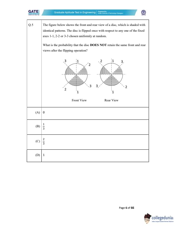


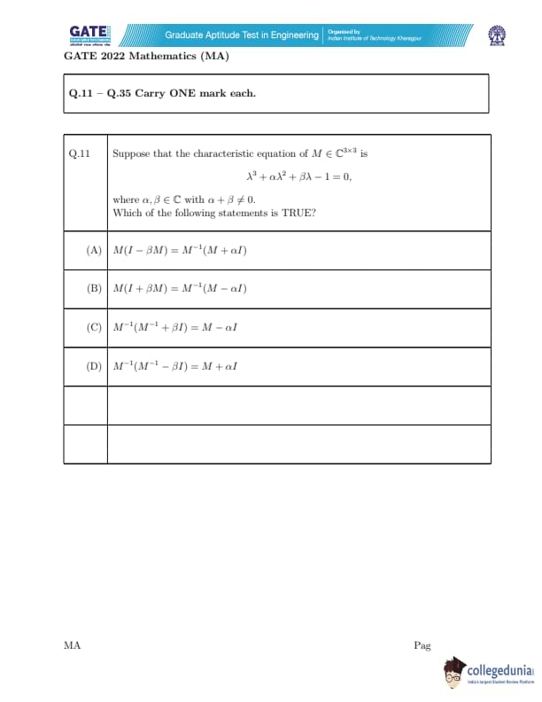
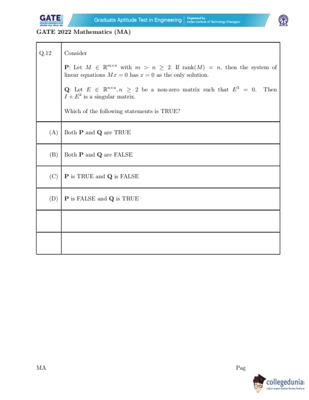
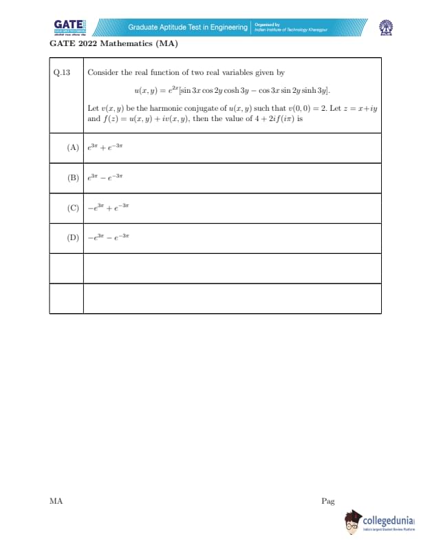
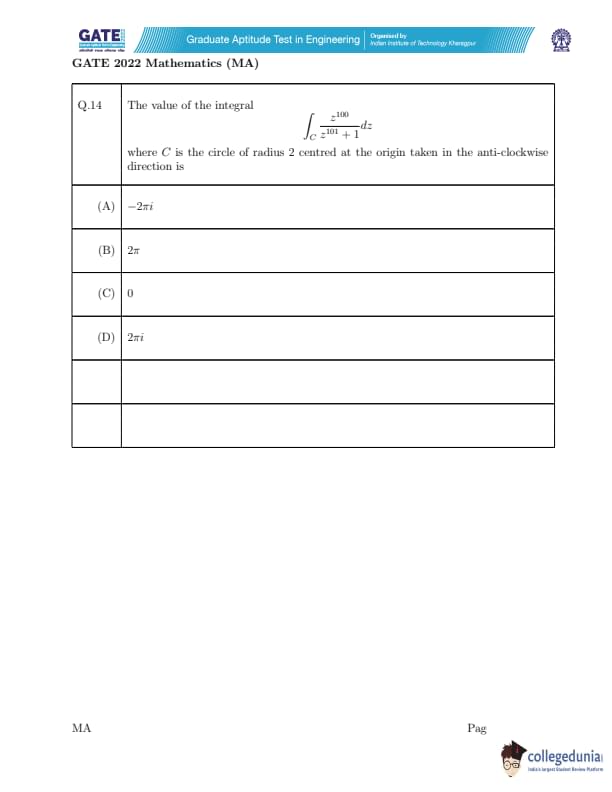
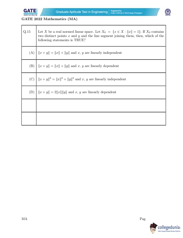
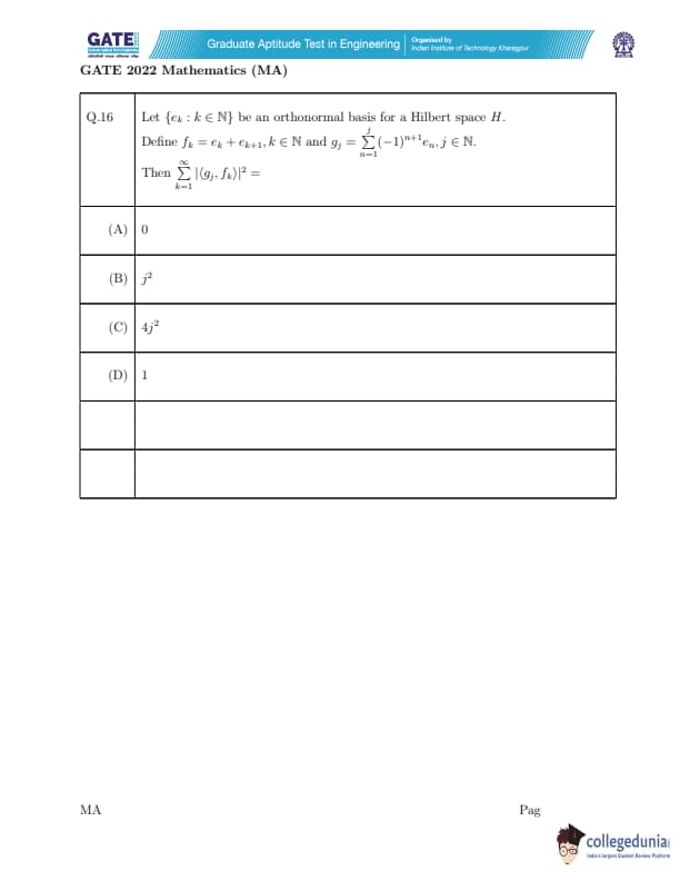
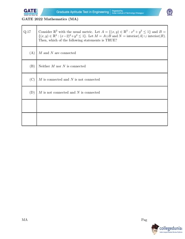
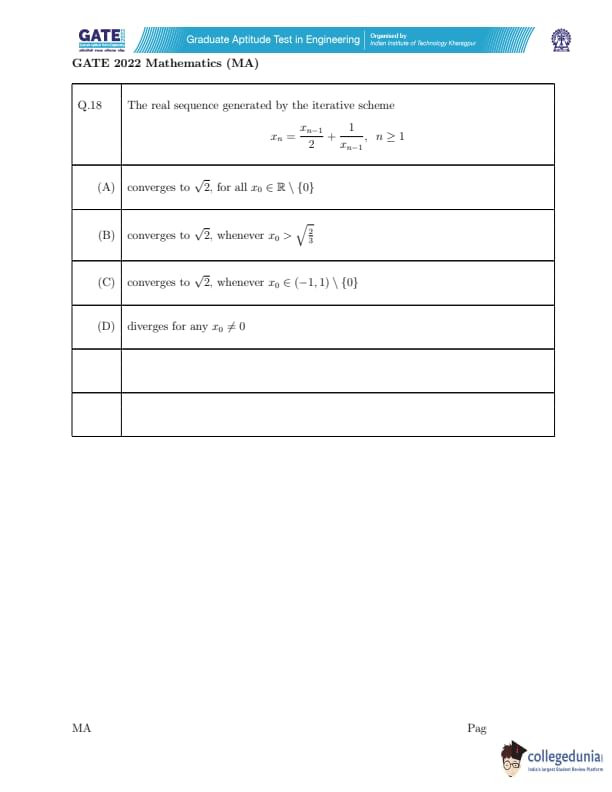

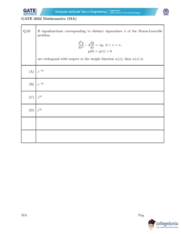
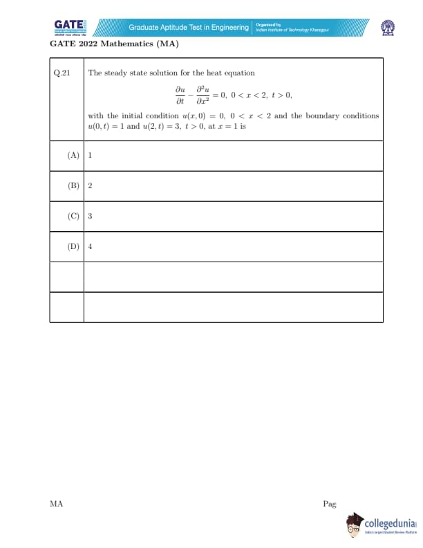
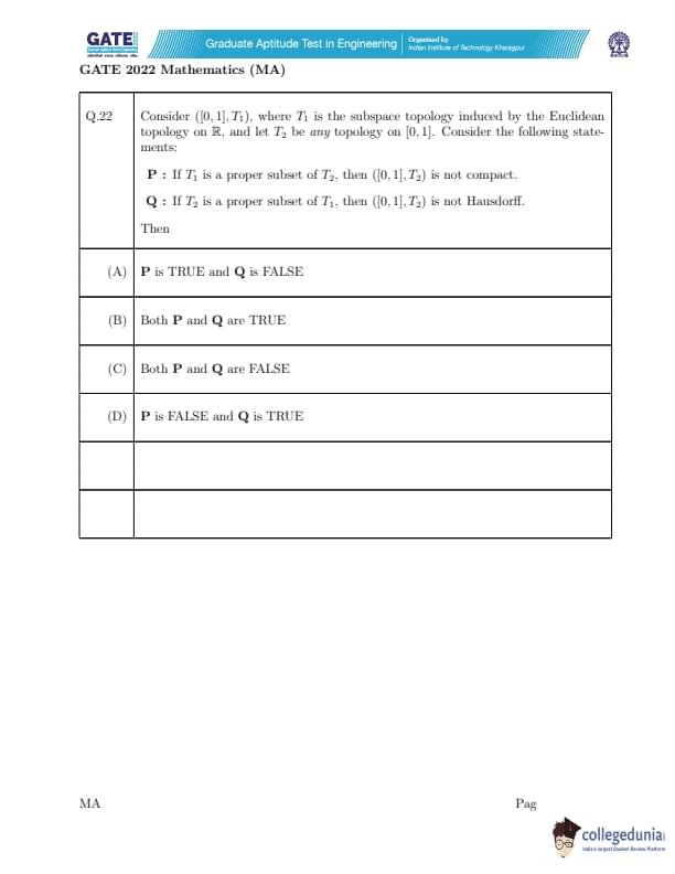
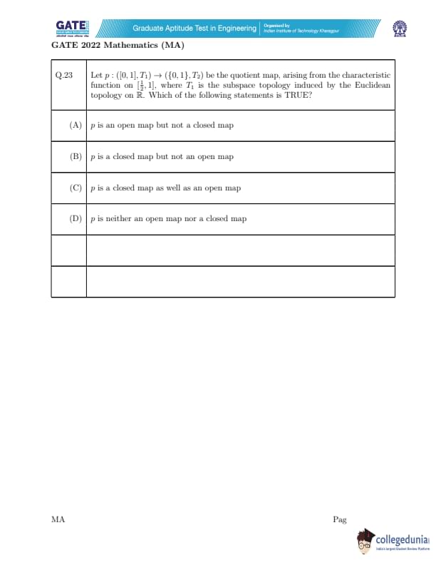

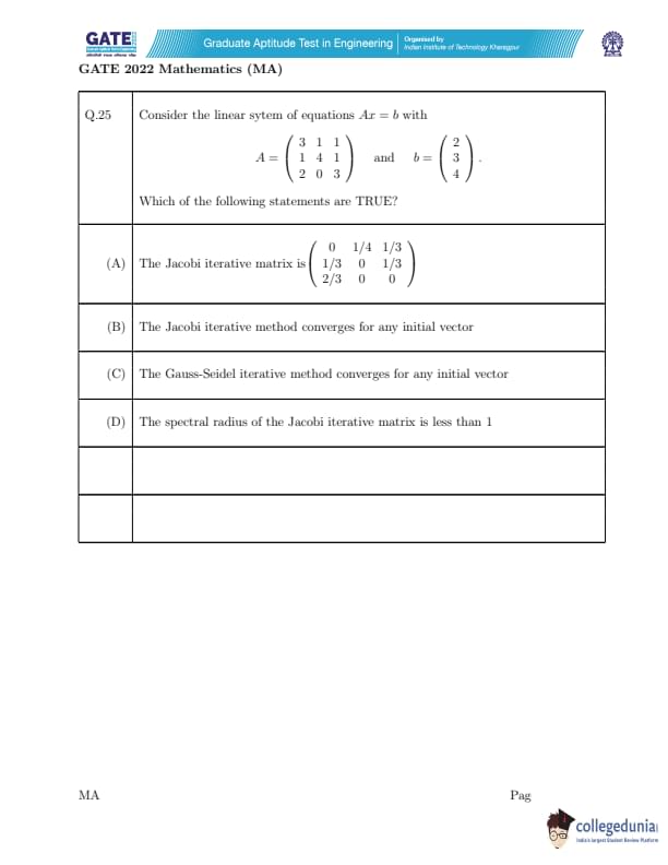


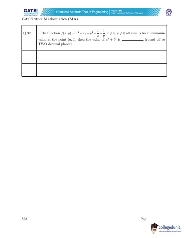
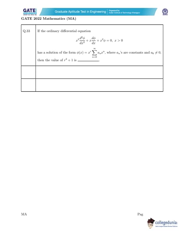
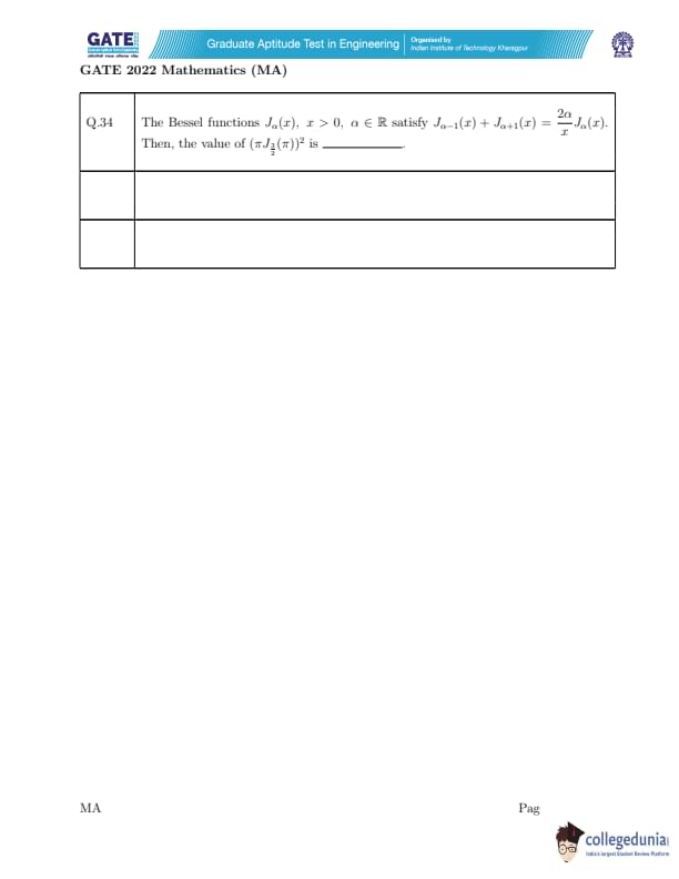
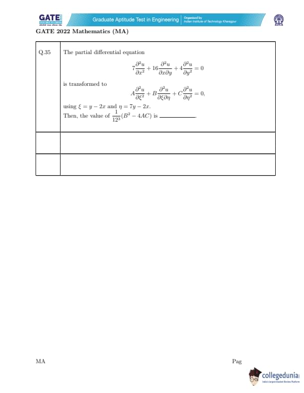
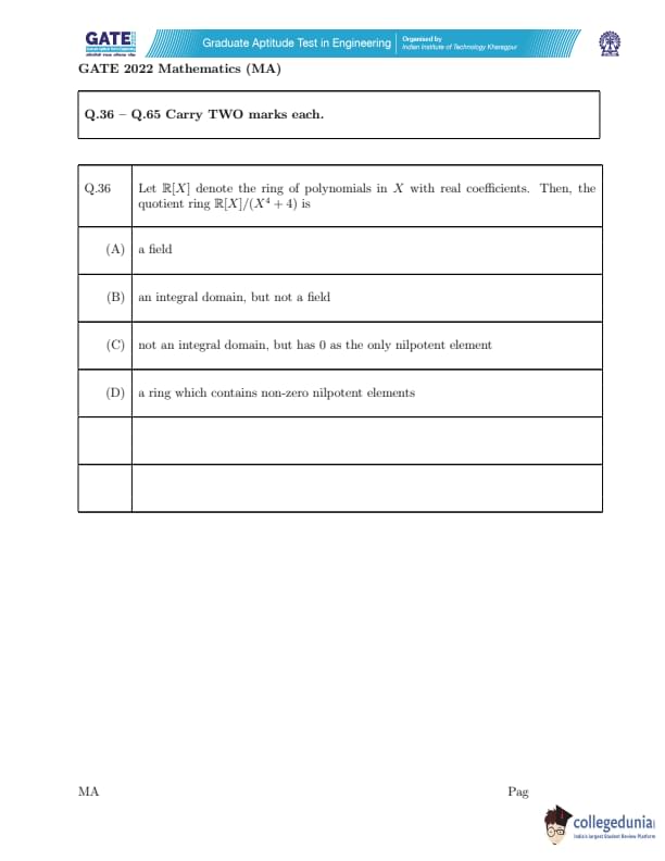
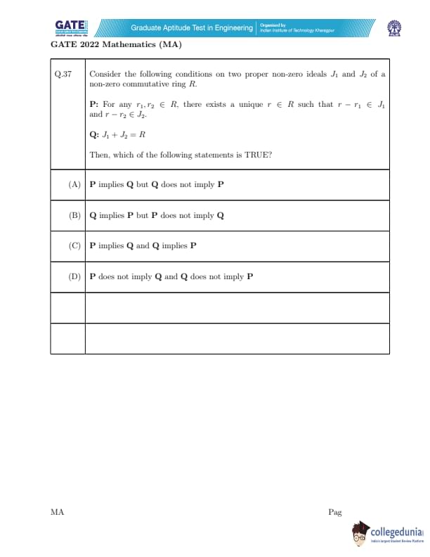
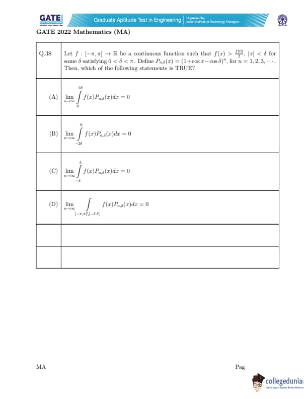
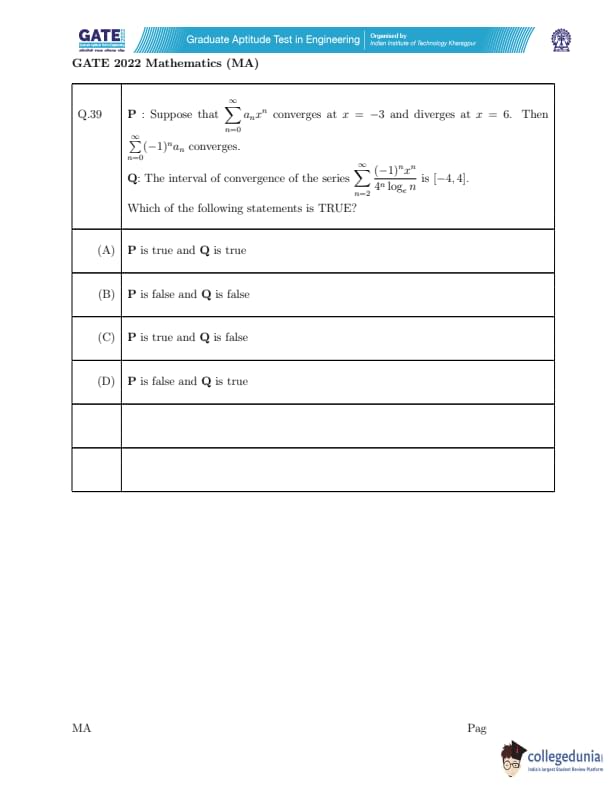
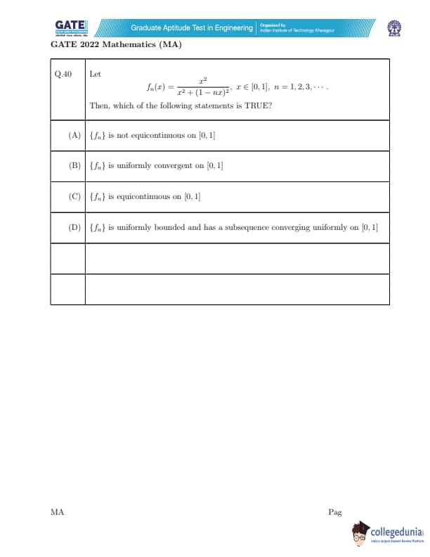
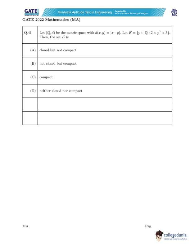
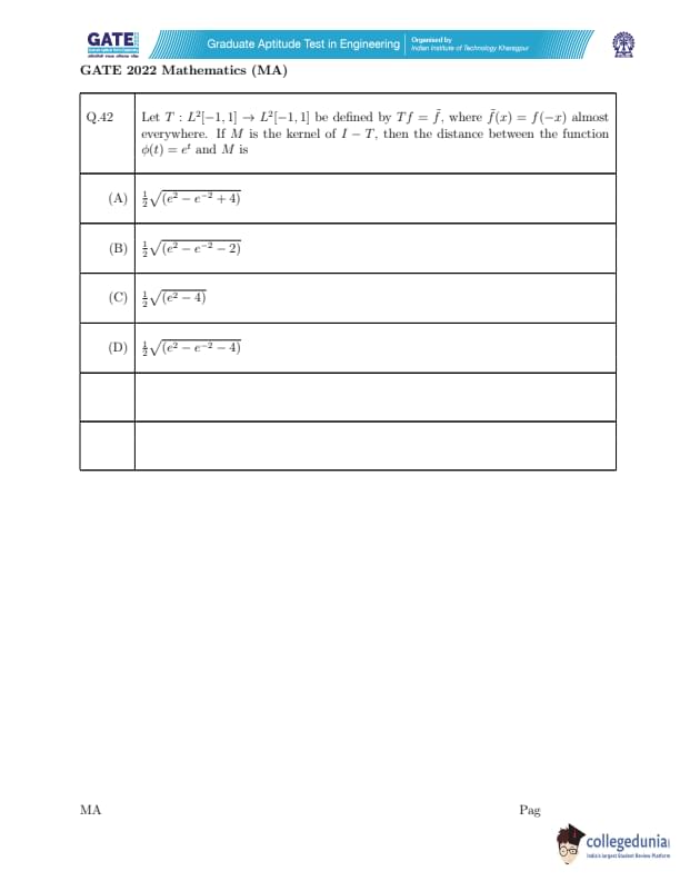
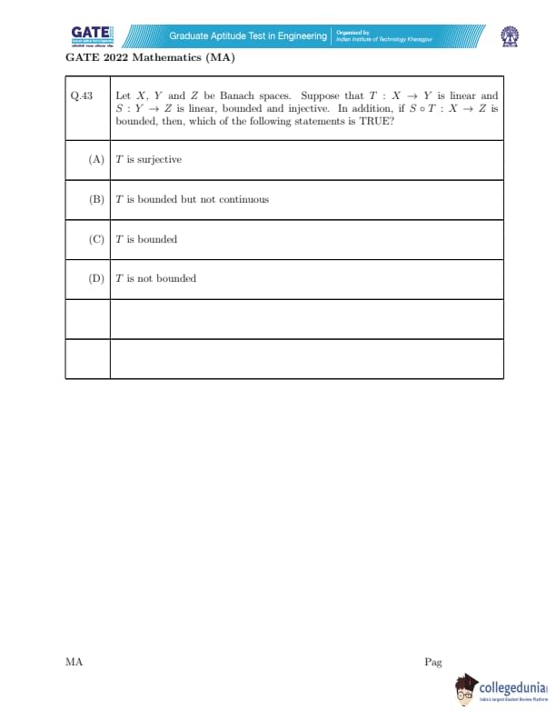
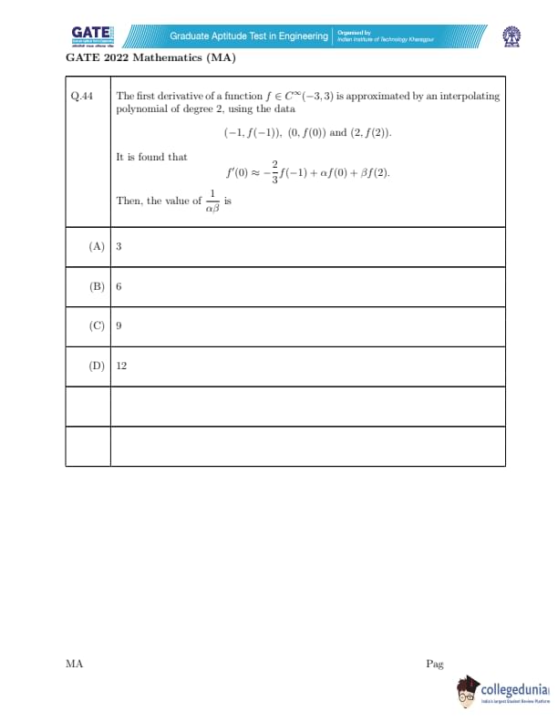

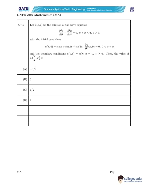

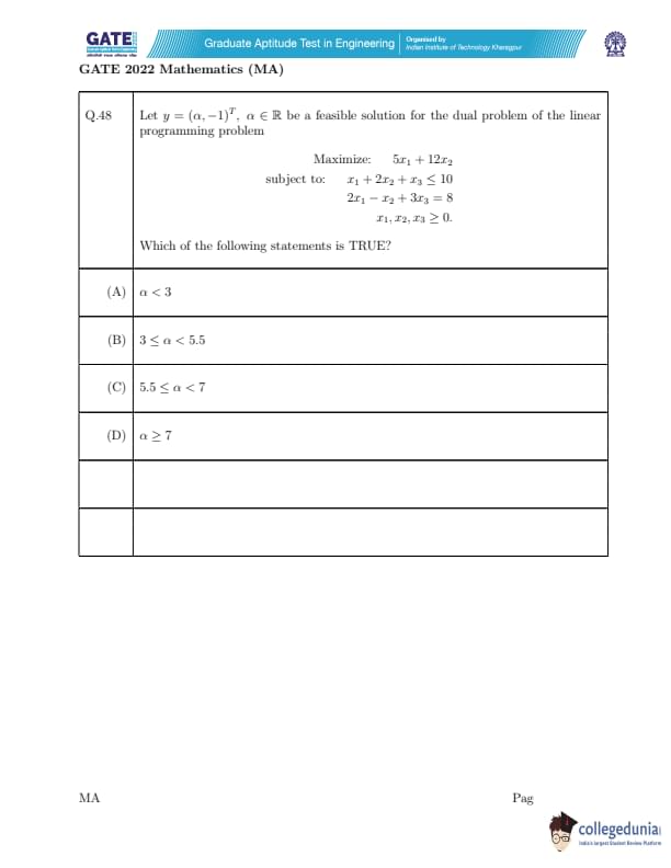
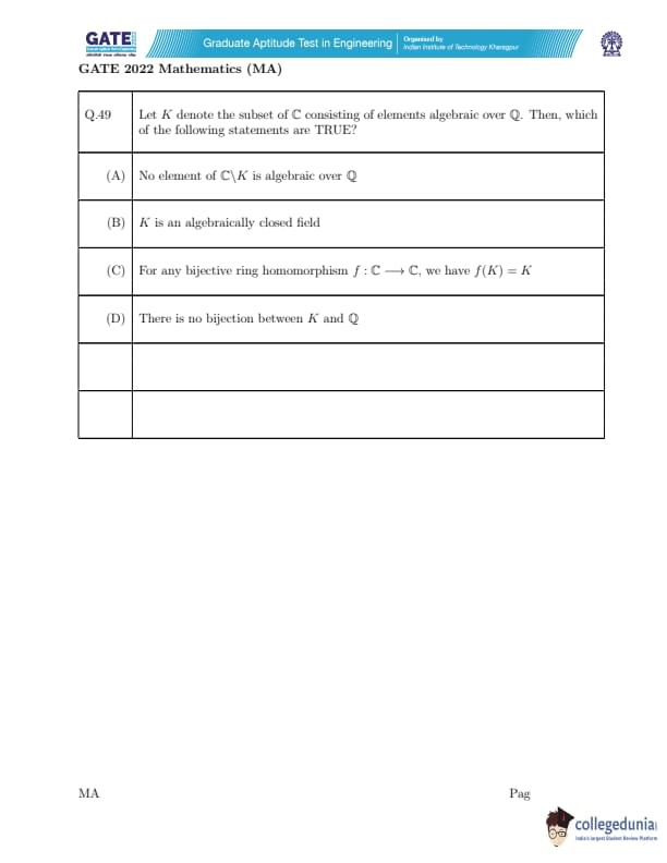
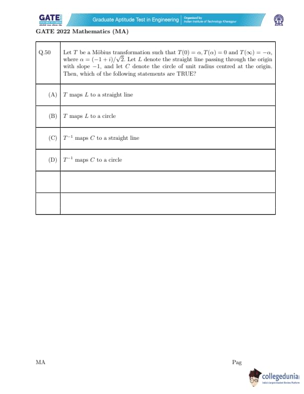
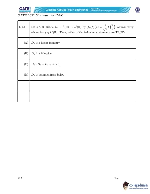
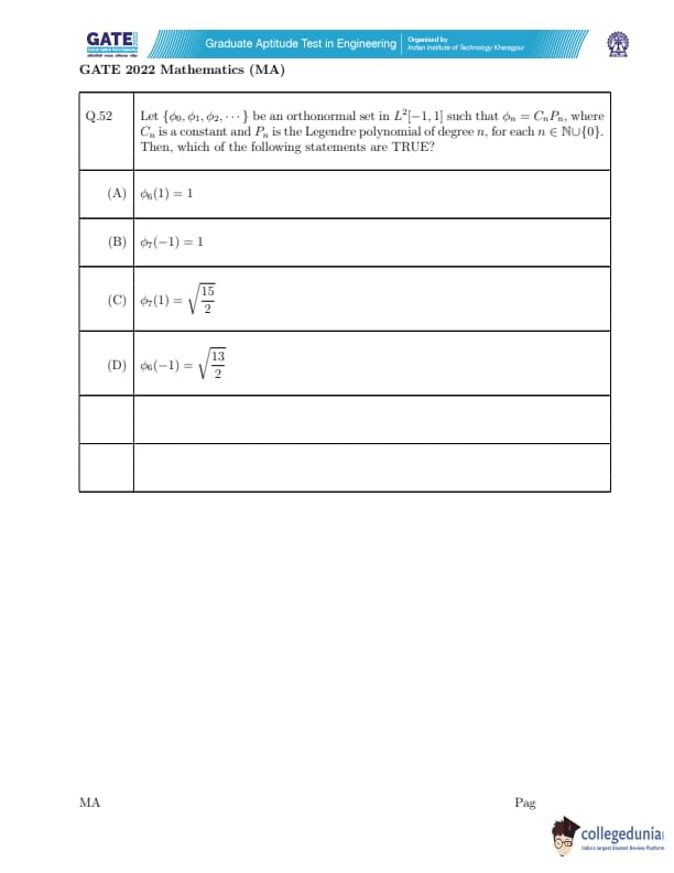
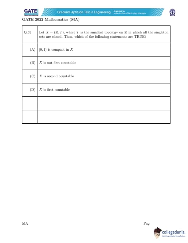
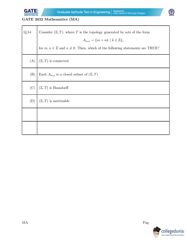
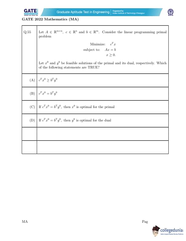
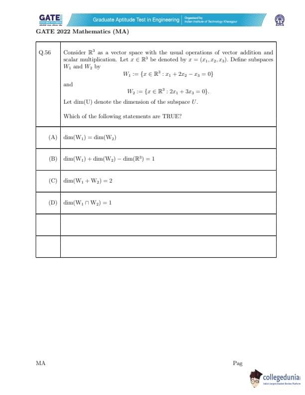
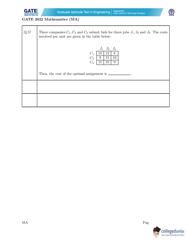
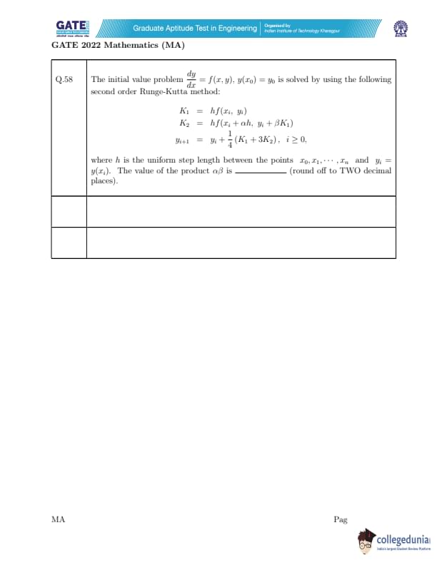

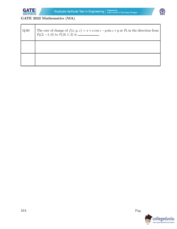
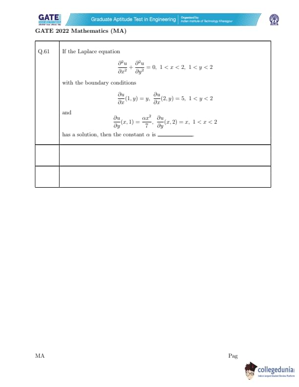
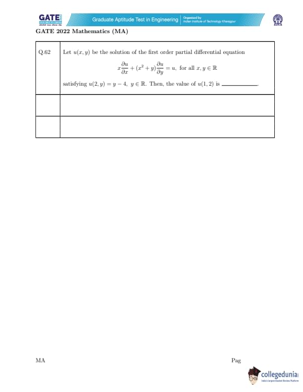
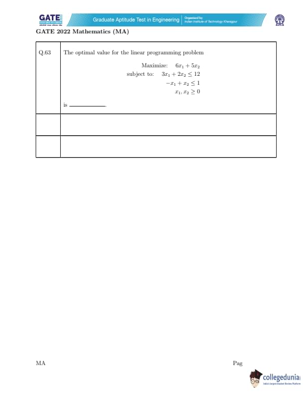
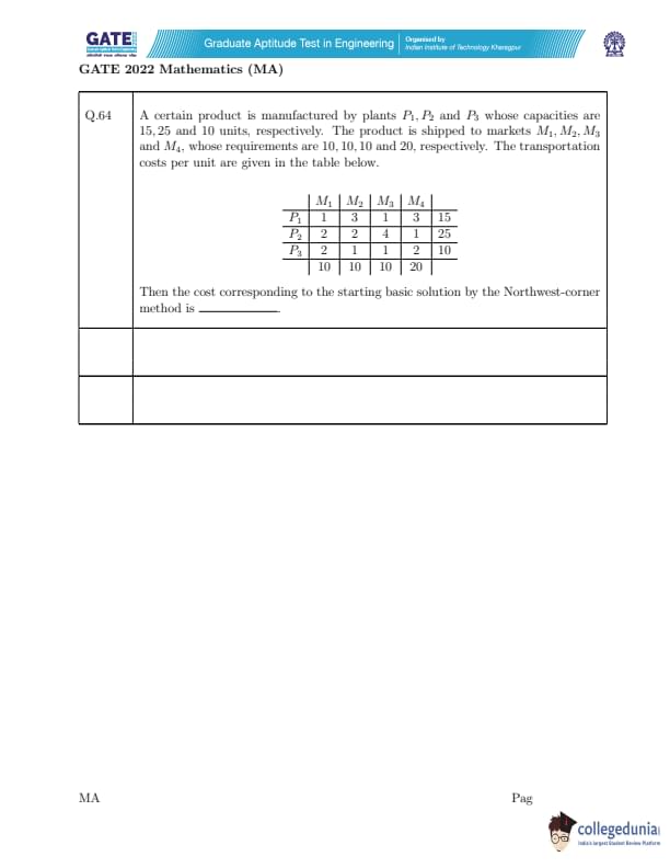

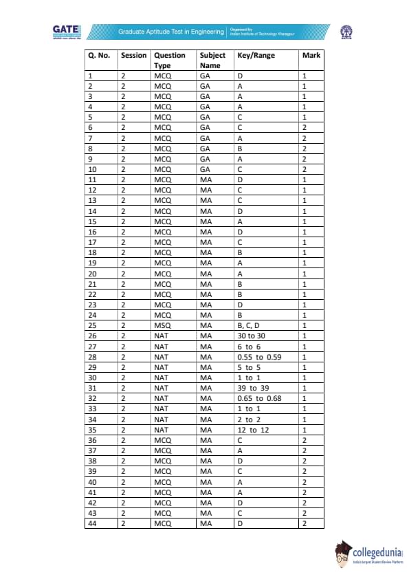
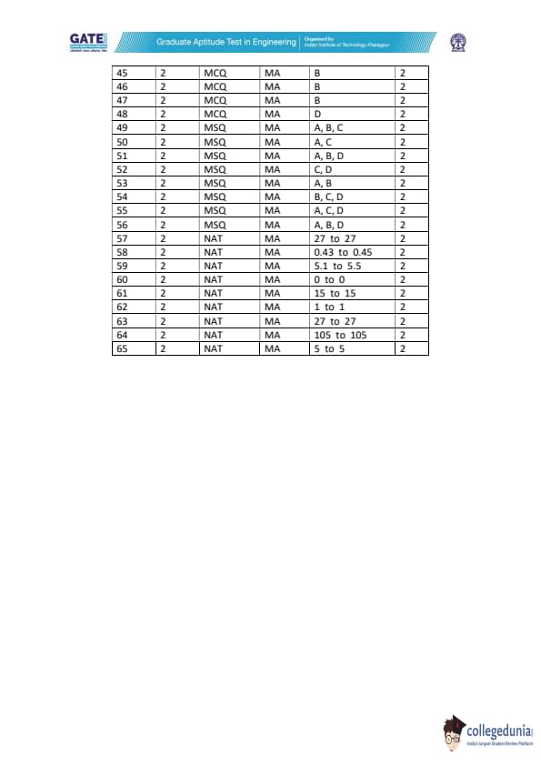
Quick Links:
GATE 2022 MA Detailed Paper Analysis
There were no changes in the overall exam pattern of GATE 2022 MA. A total of 65 questions constituted GATE 2022 MA Question Paper. Go through the below-mentioned table in order to get the details of the questions as per the carried marks-
| Question Types | Question Frequency | Carried Marks |
|---|---|---|
| No. Of 1 Mark MCQs | 19 | 19 |
| No. Of 2 Marks MCQs | 18 | 36 |
| No. Of 1 Mark NATs | 10 | 10 |
| No. Of 2 Marks NATs | 9 | 18 |
| No. Of 1 Mark MSQs | 1 | 1 |
| No. Of 2 Marks MSQs | 8 | 16 |
| Total | 65 | 100 |
- MCQs (Multiple Choice Questions) carried the maximum weightage in the exam
- There were a total of 9 MSQs (Multiple Select Questions) in the exam. 8 MSQs carried 2 marks, while only 1 MSQ carried 1 mark
- 19 out of 65 questions were NAT (Numerical Answer Type) questions.
- An attempt of 45+ questions was considered good for scoring a decent score in the examination.
Also Check:
GATE Previous Year Question Papers
| GATE 2023 Question Papers | GATE 2022 Question Papers | GATE 2021 Question Papers |
| GATE 2020 Question Papers | GATE 2019 Question Papers | GATE 2018 Question Papers |
Also Check:
Comments