CUET 2026 Mathematics May 22 Shift 1 Question Paper- Download Answer Key and Solution PDF

CUET 2026 May 22 Shift 1 Mathematics Question Paper is available for download here. NTA is conducting the CUET 2026 exam from 11th May to 31st May.

CUET 2026 Mathematics exam consists of 50 questions for 250 marks to be attempted in 60 minutes.
As per the marking scheme, 5 marks are awarded for each correct answer, and 1 mark is deducted for incorrect answer.

Candidates can download CUET 2026 May 22 Shift 1 Mathematics Question Paper with Answer Key and Solution PDF from links provided below.

Related Links:

CUET 2026 Mathematics May 22 Shift 1 Question Paper with Solution PDF

CUET May 22 Shift 1 Mathematics Question Paper 2026	Download PDF	Check Solutions

Question 1:

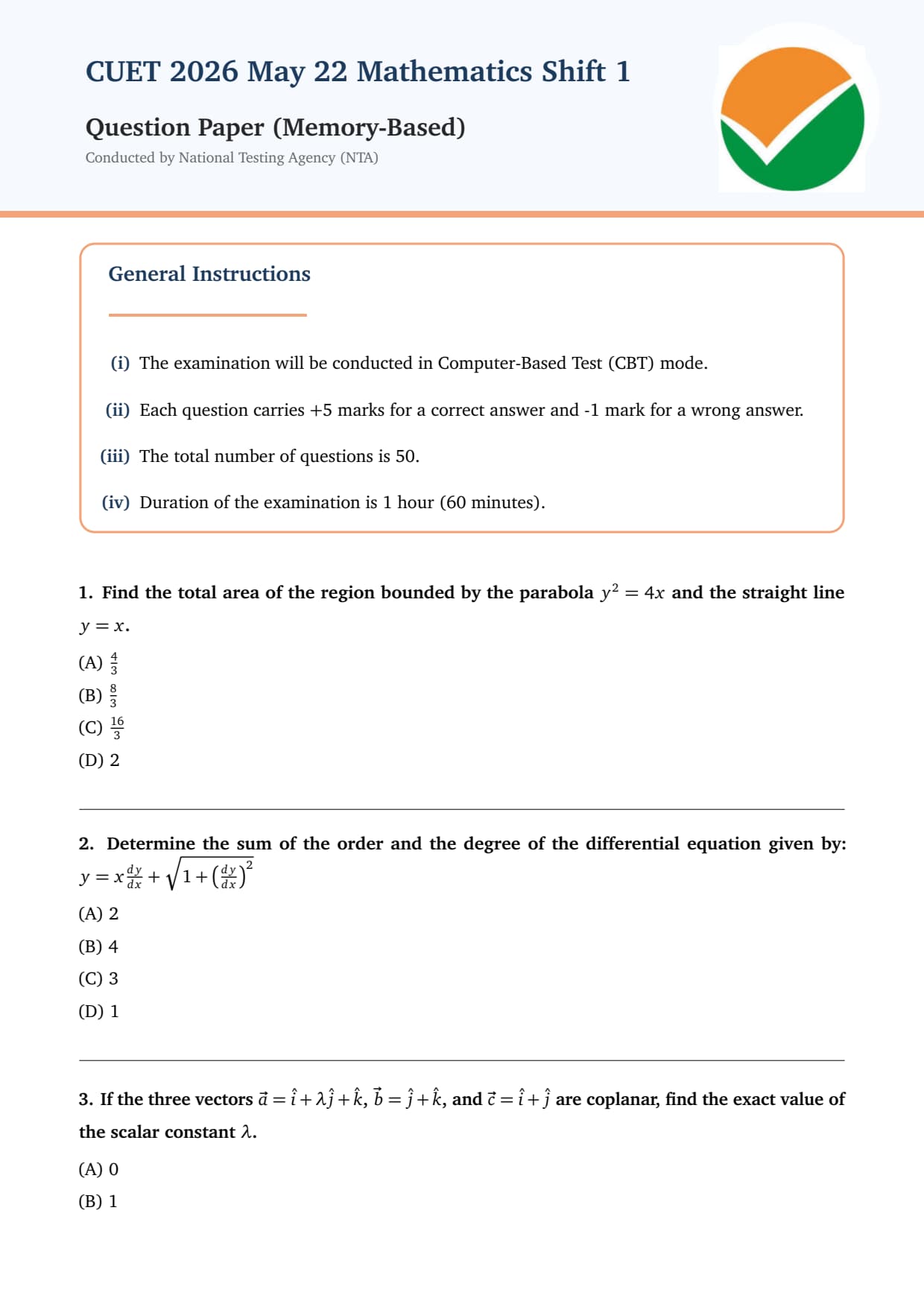
Find the total area of the region bounded by the parabola \( y^2 = 4x \) and the straight line \( y = x \).

(A) \( \frac{4}{3} \)
(B) \( \frac{8}{3} \)
(C) \( \frac{16}{3} \)
(D) \( 2 \)

Detailed Solution

Question 2:

Determine the sum of the order and the degree of the differential equation given by: \( y = x\frac{dy}{dx} + \sqrt{1 + \left(\frac{dy}{dx}\right)^2} \)

(A) \( 2 \)
(B) \( 4 \)
(C) \( 3 \)
(D) \( 1 \)

Detailed Solution

Question 3:

If the three vectors \( \vec{a} = \hat{i} + \lambda\hat{j} + \hat{k} \), \( \vec{b} = \hat{j} + \hat{k} \), and \( \vec{c} = \hat{i} + \hat{j} \) are coplanar, find the exact value of the scalar constant \( \lambda \).

(A) \( 0 \)
(B) \( 1 \)
(C) \( -2 \)
(D) \( 2 \)

Detailed Solution

Question 4:

A straight vector line makes equal acute angles \( \alpha = \beta = \gamma \) with all three primary coordinate axes. Find the absolute value of \( \cos\alpha \).

(A) \( \frac{1}{\sqrt{3}} \)
(B) \( \frac{1}{3} \)
(C) \( \frac{1}{\sqrt{2}} \)
(D) \( 1 \)

Detailed Solution

Question 5:

Simplify the inverse trigonometric expression to find its principal value: \( \tan^{-1}\left(\frac{1}{2}\right) + \tan^{-1}\left(\frac{1}{3}\right) \)

(A) \( \frac{\pi}{2} \)
(B) \( \tan^{-1}\left(\frac{2}{5}\right) \)
(C) \( \frac{\pi}{3} \)
(D) \( \frac{\pi}{4} \)

Detailed Solution

Question 6:

Under what condition will a linear programming system containing objective function variables have no common feasible region?

(A) When the objective function coefficients are set strictly to zero.
(B) When the system of linear constraints is mutually inconsistent, meaning there is no overlapping coordinate space that satisfies all conditions at once.
(C) When all constraints are written using strictly non-negative bounding limits.
(D) When the optimal solution point matches one of the outer corner coordinates.

Detailed Solution

Question 7:

Find the total area of the region bounded between the curve \( y = x^3 \), the x-axis, and the vertical lines \( x = -1 \) and \( x = 1 \).

(A) \( 0 \)
(B) \( \frac{1}{4} \)
(C) \( \frac{1}{2} \)
(D) \( 1 \)

Detailed Solution

Question 8:

Determine the degree of the following differential equation: \( \left[1 + \left(\frac{dy}{dx}\right)^2\right]^{\frac{3}{2}} = \frac{d^2y}{dx^2} \)

(A) Not defined
(B) \( 2 \)
(C) \( 3 \)
(D) \( 1 \)

Detailed Solution

Question 9:

If the straight line equation \( \frac{x-1}{2} = \frac{y-2}{3} = \frac{z-3}{4} \) runs completely parallel to the plane surface given by \( A x + 2y + 3z = 5 \), find the value of the coefficient \( A \).

(A) \( 9 \)
(B) \( 0 \)
(C) \( -9 \)
(D) \( -4 \)

Detailed Solution

Question 10:

Find the maximum value of the linear objective function \( Z = 3x + 4y \) subject to the system constraints: \( x + y \le 4 \), \( x \ge 0 \), and \( y \ge 0 \).

(A) \( 12 \)
(B) \( 16 \)
(C) \( 24 \)
(D) \( 0 \)

Detailed Solution

CUET UG 2026 Exam Pattern

Parameter	Details
Exam Name	Common University Entrance Test (CUET UG) 2026
Conducting Body	National Testing Agency (NTA)
Exam Mode	Computer-Based Test (CBT)
Exam Duration	60 minutes per test
Total Sections	3 (Languages, Domain Subjects, General Test)
Question Type	Multiple Choice Questions (MCQs)
Questions per Test	50 questions (all compulsory)
Marking Scheme	+5 for correct, -1 for incorrect
Maximum Marks	250 marks per test
Maximum Subject Choices	5 subjects in total
Syllabus Base	Class 12 NCERT (mainly for Domain Subjects)

CUET UG 2026 Paper Analysis

CUET Questions

1.
M is a square matrix of order 3. If \[ M(\operatorname{adj} M)= \begin{bmatrix} 5 & 0 & 0 \\ 0 & 5 & 0 \\ 0 & 0 & 5 \end{bmatrix}, \] then the value of \[ |M+\operatorname{adj} M| \] is equal to:

\( 125 \)
\( 30 \)
\( 25 \)
\( 50 \)

View Solution

2.
If \( P(A) = \frac{3}{5} \), \( P(\overline{B}) = \frac{4}{7} \), and \( P(A \cup B) = \frac{2}{3} \), which of the following are correct?

(A) \( P(A \cap B) = \frac{17}{105} \)
(B) \( P(A \mid B) = \frac{17}{45} \)
(C) A and B are independent events
(D) \( P(B \mid A) = \frac{17}{36} \)

(A), (B) and (D) only
(B) and (C) only
(A) and (D) only
(A) and (B) only

View Solution

3.
For the function \[ f(x)=ax+\frac{b}{x}, \qquad a>0,\; b>0, \] which of the following statements are correct?

(A) Function \(f(x)\) is increasing on \[ \left(\sqrt{\frac{b}{a}},\,\infty\right) \]

(B) Function \(f(x)\) is increasing on \[ (-\infty,\infty) \]

(C) Function \(f(x)\) is decreasing on \[ \left(-\sqrt{\frac{b}{a}},\,\sqrt{\frac{b}{a}}\right) \]

(D) Function \(f(x)\) is increasing on \[ \left(-\infty,\,-\sqrt{\frac{b}{a}}\right) \]

(A), (B) and (D) only
(A) and (C) only
(A), (C) and (D) only
(A) and (D) only

View Solution

4.
The order of the differential equation \[ \left(\frac{d^5y}{dx^5}\right)^2 + \frac{dy}{dx} + y^2 = 0 \] is:

1
Not defined
5
2

View Solution

5.
Simplify the inverse trigonometric expression to find its principal value: \[ \tan^{-1}\left(\frac{1}{2}\right) + \tan^{-1}\left(\frac{1}{3}\right) \]

\( \frac{\pi}{2} \)
\( \tan^{-1}\left(\frac{2}{5}\right) \)
\( \frac{\pi}{3} \)
\( \frac{\pi}{4} \)

View Solution

6.
If \( A=\begin{bmatrix}2 & 3 \\ 5 & -2\end{bmatrix} \), then:

\( A^{-1}=\frac{1}{11}A \)
\( A^{-1}=\frac{1}{19}A \)
\( A^{-1}=-\frac{1}{19}A \)
\( A^{-1}=\frac{1}{7}A \)

View Solution

CUET 2026 Mathematics May 22 Shift 1 Question Paper- Download Answer Key and Solution PDF

CUET 2026 Mathematics May 22 Shift 1 Question Paper with Solution PDF

CUET UG 2026 Exam Pattern

CUET UG 2026 Paper Analysis

CUET Questions

1.
M is a square matrix of order 3. If \[ M(\operatorname{adj} M)= \begin{bmatrix} 5 & 0 & 0 \\ 0 & 5 & 0 \\ 0 & 0 & 5 \end{bmatrix}, \] then the value of \[ |M+\operatorname{adj} M| \] is equal to:

2.
If \( P(A) = \frac{3}{5} \), \( P(\overline{B}) = \frac{4}{7} \), and \( P(A \cup B) = \frac{2}{3} \), which of the following are correct?

(A) \( P(A \cap B) = \frac{17}{105} \)
(B) \( P(A \mid B) = \frac{17}{45} \)
(C) A and B are independent events
(D) \( P(B \mid A) = \frac{17}{36} \)

4.
The order of the differential equation \[ \left(\frac{d^5y}{dx^5}\right)^2 + \frac{dy}{dx} + y^2 = 0 \] is:

5.
Simplify the inverse trigonometric expression to find its principal value: \[ \tan^{-1}\left(\frac{1}{2}\right) + \tan^{-1}\left(\frac{1}{3}\right) \]

6.
If \( A=\begin{bmatrix}2 & 3 \\ 5 & -2\end{bmatrix} \), then:

Comments

SUBSCRIBE TO OUR NEWS LETTER

CUET 2026 Mathematics May 22 Shift 1 Question Paper with Solution PDF

CUET UG 2026 Exam Pattern

CUET UG 2026 Paper Analysis

CUET Questions

1.M is a square matrix of order 3. If \[ M(\operatorname{adj} M)= \begin{bmatrix} 5 & 0 & 0 \\ 0 & 5 & 0 \\ 0 & 0 & 5 \end{bmatrix}, \] then the value of \[ |M+\operatorname{adj} M| \] is equal to:

2.If \( P(A) = \frac{3}{5} \), \( P(\overline{B}) = \frac{4}{7} \), and \( P(A \cup B) = \frac{2}{3} \), which of the following are correct? (A) \( P(A \cap B) = \frac{17}{105} \) (B) \( P(A \mid B) = \frac{17}{45} \) (C) A and B are independent events (D) \( P(B \mid A) = \frac{17}{36} \)

4.The order of the differential equation \[ \left(\frac{d^5y}{dx^5}\right)^2 + \frac{dy}{dx} + y^2 = 0 \] is:

5.Simplify the inverse trigonometric expression to find its principal value: \[ \tan^{-1}\left(\frac{1}{2}\right) + \tan^{-1}\left(\frac{1}{3}\right) \]

6.If \( A=\begin{bmatrix}2 & 3 \\ 5 & -2\end{bmatrix} \), then:

Comments

SUBSCRIBE TO OUR NEWS LETTER

1.
M is a square matrix of order 3. If \[ M(\operatorname{adj} M)= \begin{bmatrix} 5 & 0 & 0 \\ 0 & 5 & 0 \\ 0 & 0 & 5 \end{bmatrix}, \] then the value of \[ |M+\operatorname{adj} M| \] is equal to:

2.
If \( P(A) = \frac{3}{5} \), \( P(\overline{B}) = \frac{4}{7} \), and \( P(A \cup B) = \frac{2}{3} \), which of the following are correct?

(A) \( P(A \cap B) = \frac{17}{105} \)
(B) \( P(A \mid B) = \frac{17}{45} \)
(C) A and B are independent events
(D) \( P(B \mid A) = \frac{17}{36} \)

4.
The order of the differential equation \[ \left(\frac{d^5y}{dx^5}\right)^2 + \frac{dy}{dx} + y^2 = 0 \] is:

5.
Simplify the inverse trigonometric expression to find its principal value: \[ \tan^{-1}\left(\frac{1}{2}\right) + \tan^{-1}\left(\frac{1}{3}\right) \]

6.
If \( A=\begin{bmatrix}2 & 3 \\ 5 & -2\end{bmatrix} \), then: