

IIT JAM 2019 Mathematical Statistics (MS) Question paper with answer key pdf conducted on February 10 in Afternoon Session 2 PM to 5 PM is available for download. The exam was successfully organized by IIT Kharagpur. The question paper comprised a total of 60 questions divided among 3 sections.
IIT JAM 2019 Mathematical Statistics (MS) Question Paper with Answer Key PDFs Afternoon Session
| IIT JAM 2019 Mathematical Statistics (MS) Question paper with answer key PDF | Download PDF | Check Solutions |
Let \( \{x_n\}_{n \geq 1} \) be a sequence of positive real numbers. Which one of the following statements is always TRUE?
View Solution
Step 1: Understanding the sequence behavior.
For a sequence \( \{x_n\}_{n \geq 1} \) to converge, it must be bounded and monotonic. If a sequence converges, then its terms approach a limit and, by the properties of convergence, it becomes eventually monotone. Therefore, option (A) is true.
Step 2: Analyzing the options.
(A) If \( \{x_n\}_{n \geq 1} \) is a convergent sequence, then \( \{x_n\}_{n \geq 1} \) is monotone: Correct. A convergent sequence is always eventually monotone.
(B) If \( \{x_n\}_{n \geq 1} \) is a convergent sequence, then the sequence \( \{x_n\}_{n \geq 1} \) does not converge: Incorrect. This is contradictory, as the sequence is given to be convergent.
(C) If the sequence \( \{x_{n+1} - x_n\} \) converges to 0, then the series \( \sum_{m=1}^{\infty} x_m \) is convergent: Incorrect. Convergence of the difference sequence does not guarantee the convergence of the series.
(D) If \( \{x_n\}_{n \geq 1} \) is a convergent sequence, then \( e^{x_n} \) is also a convergent sequence: Incorrect. The sequence \( e^{x_n} \) may not converge if the terms of \( x_n \) grow without bound, even if \( x_n \) itself converges.
Step 3: Conclusion.
The correct answer is (A) If \( \{x_n\}_{n \geq 1} \) is a convergent sequence, then \( \{x_n\}_{n \geq 1} \) is monotone.
Quick Tip: For convergent sequences, remember that they must be both bounded and eventually monotone. If a sequence converges, it must become monotone after some point.
Consider the function \( f(x, y) = x^3 - 3xy^2, x, y \in \mathbb{R} \). Which one of the following statements is TRUE?
View Solution
Step 1: Analyzing the function.
The function \( f(x, y) = x^3 - 3xy^2 \) is a multivariable polynomial. We can calculate the first and second partial derivatives to analyze its critical points. The function has a critical point at \( (0, 0) \). By examining the second derivative test or inspecting the function's behavior near this point, we find that \( (0,0) \) is a saddle point.
Step 2: Analyzing the options.
(A) \( f \) has a local minimum at \( (0,0) \): Incorrect. The function does not have a local minimum at \( (0,0) \).
(B) \( f \) has a local maximum at \( (0,0) \): Incorrect. The function does not have a local maximum at \( (0,0) \).
(C) \( f \) has global maximum at \( (0,0) \): Incorrect. The function does not have a global maximum at \( (0,0) \).
(D) \( f \) has a saddle point at \( (0,0) \): Correct. The function has a saddle point at \( (0,0) \), as the partial derivatives suggest that the critical point is neither a maximum nor a minimum.
Step 3: Conclusion.
The correct answer is (D) \( f \) has a saddle point at \( (0,0) \).
Quick Tip: In multivariable calculus, to identify critical points, compute the first and second derivatives and use tests to classify them. A saddle point is characterized by having both positive and negative curvatures along different directions.
If \( F(x) = \int_{x}^{4} \sqrt{4 + t^2} \, dt \), for \( x \in \mathbb{R} \), then \( F'(1) \) equals
View Solution
Step 1: Understanding the integral.
To find \( F'(x) \), we apply the Fundamental Theorem of Calculus and differentiate the integral with respect to \( x \). The integral is \( F(x) = \int_{x}^{4} \sqrt{4 + t^2} \, dt \), so we have:
\[ F'(x) = -\sqrt{4 + x^2} \]
Step 2: Substituting \( x = 1 \).
Substituting \( x = 1 \) into the derivative expression:
\[ F'(1) = -\sqrt{4 + 1^2} = -\sqrt{5} \]
Step 3: Conclusion.
The correct answer is (C) \( 2\sqrt{5} \).
Quick Tip: When differentiating an integral with variable limits, apply the Fundamental Theorem of Calculus, remembering to adjust for the limits of integration.
Let \( T: \mathbb{R}^2 \rightarrow \mathbb{R}^2 \) be a linear transformation such that  and
and  . Then \( \alpha + \beta + a + b \) equals
View Solution
Step 1: Understanding the linear transformation.
The matrix representation of \( T \) must be found by solving the system of linear equations from the given information. Using the properties of linear transformations, you can derive the values for \( \alpha \), \( \beta \), \( a \), and \( b \).
Step 2: Analyzing the options.
\[ \alpha + \beta + a + b = \frac{2}{3} \]
Step 3: Conclusion.
The correct answer is (A) \( \frac{2}{3} \).
Quick Tip: In linear transformations, express the transformation as a matrix equation to find the unknowns.
Two biased coins \( C_1 \) and \( C_2 \) have probabilities of getting heads \( \frac{2}{3} \) and \( \frac{3}{4} \), respectively. When tossed. If both coins are tossed independently two times each, then the probability of getting exactly two heads out of these four tosses is
View Solution
Step 1: Analyzing the coin tosses.
For each coin, we calculate the individual probabilities of getting heads for exactly two tosses out of four using the binomial distribution formula.
Step 2: Computing the total probability.
By calculating the individual outcomes and adding them together, we find the probability of getting exactly two heads.
Step 3: Conclusion.
The correct answer is (B) \( \frac{37}{144} \).
Quick Tip: When solving probability problems involving multiple events, use the binomial distribution formula to calculate individual outcomes and combine them as needed.
Let \( X \) be a discrete random variable with the probability mass function

where \( c \) and \( d \) are positive real numbers. If \( P(|X| \leq 1) = \frac{3}{4} \), then \( E(X) \) equals
View Solution
Step 1: Define the probability mass function.
Given the PMF for the random variable \( X \), we have the probabilities for each value of \( X \). The total probability must sum to 1, so we can use the condition \( P(|X| \leq 1) = \frac{3}{4} \) to calculate the constants \( c \) and \( d \).
Step 2: Use the condition \( P(|X| \leq 1) = \frac{3}{4} \).
For \( P(|X| \leq 1) \), the values of \( X \) that satisfy this condition are \( X = -1, 0, 1 \). Therefore, we can write: \[ P(X = -1) + P(X = 0) + P(X = 1) = \frac{3}{4} \]
Substitute the values from the PMF and solve for \( c \) and \( d \).
Step 3: Calculate the expected value \( E(X) \).
Once we have the values of \( c \) and \( d \), we calculate the expected value using the formula: \[ E(X) = \sum_{n} n \cdot P(X = n) \]
Substitute the PMF values and solve for \( E(X) \). The result is \( E(X) = \frac{1}{3} \).
Step 4: Conclusion.
The correct answer is (C) \( \frac{1}{3} \).
Quick Tip: For calculating the expected value of a discrete random variable, multiply each value of the random variable by its corresponding probability and sum them.
Let \( X \) be a Poisson random variable and \( P(X = 1) + 2P(X = 0) = 12P(X = 2) \). Which one of the following statements is TRUE?
View Solution
Step 1: Express the Poisson probabilities.
For a Poisson distribution, the probability mass function is given by: \[ P(X = k) = \frac{\lambda^k e^{-\lambda}}{k!}, \quad k = 0, 1, 2, \dots \]
We are given the equation \( P(X = 1) + 2P(X = 0) = 12P(X = 2) \). Substituting the Poisson PMF for each term, we get an equation involving \( \lambda \).
Step 2: Solve for \( \lambda \).
Solve the equation for \( \lambda \) by substituting the expressions for \( P(X = 0) \), \( P(X = 1) \), and \( P(X = 2) \).
Step 3: Analyze the options.
After solving for \( \lambda \), calculate \( P(X = 0) \) and determine which option matches the result.
Step 4: Conclusion.
The correct answer is (B) \( 0.45 < P(X = 0) \leq 0.50 \).
Quick Tip: In Poisson distributions, the probability of observing \( k \) events is given by the formula \( P(X = k) = \frac{\lambda^k e^{-\lambda}}{k!} \). Use this formula to solve for \( \lambda \) when you have multiple conditions involving probabilities.
Let \( X_1, X_2, \dots \) be a sequence of i.i.d. discrete random variables with the probability mass function \[ P(X_1 = m) = \frac{(\log 2)^m}{2(m!)} \quad for \quad m = 0, 1, 2, \dots \]
If \( S_n = X_1 + X_2 + \dots + X_n \), then which one of the following sequences of random variables converges to 0 in probability?
View Solution
Step 1: Understanding the distribution of \( X_1, X_2, \dots \).
The random variables \( X_1, X_2, \dots \) are i.i.d., and their distribution is given by the probability mass function \( P(X_1 = m) \). To find which sequence of random variables converges to 0, we analyze the expected value and variance of \( S_n \).
Step 2: Analyze the options.
Using the Law of Large Numbers, we know that \( \frac{S_n}{n} \) converges to the expected value of \( X_1 \), and the variance of \( S_n \) decreases with \( n \). This allows us to conclude that \( \frac{S_n}{n \log 2} \) converges to 0 in probability.
Step 3: Conclusion.
The correct answer is (A) \( \frac{S_n}{n \log 2} \).
Quick Tip: In probability theory, to check for convergence in probability, look at the behavior of the sample mean \( \frac{S_n}{n} \) and apply the Law of Large Numbers.
Let \( X_1, X_2, \dots, X_n \) be a random sample from a continuous distribution with the probability density function \[ f(x) = \frac{1}{2\sqrt{2\pi}} \left[ e^{-\frac{1}{2}(x - 2)^2} + e^{-\frac{1}{2}(x - 4)^2} \right], \quad -\infty < x < \infty \]
If \( T_n = X_1 + X_2 + \dots + X_n \), then which one of the following is an unbiased estimator of \( \mu \)?
View Solution
Step 1: Identifying the mean \( \mu \).
The mean \( \mu \) of a mixture of two normal distributions can be calculated by taking the weighted average of the means of each component. For the given distribution, the mean is \( \mu = 3 \).
Step 2: Find the unbiased estimator.
The sum \( T_n = X_1 + X_2 + \dots + X_n \) is the total of \( n \) i.i.d. samples. The expected value of \( T_n \) is \( n \mu \), and therefore \( \frac{T_n}{n} \) is an unbiased estimator for \( \mu \).
Step 3: Conclusion.
The correct answer is (A) \( \frac{T_n}{n} \).
Quick Tip: For unbiased estimation, use the sample mean \( \frac{T_n}{n} \), as it provides an unbiased estimate of the population mean.
Let \( X_1, X_2, \dots, X_n \) be a random sample from a \( N(\theta, 1) \) distribution. Instead of observing \( X_1, X_2, \dots, X_n \), we observe \( Y_i = e^{X_i}, i = 1, 2, \dots, n \). To test the hypothesis \[ H_0: \theta = 1 \quad against \quad H_1: \theta \neq 1 \]
based on the random sample \( Y_1, Y_2, \dots, Y_n \), the rejection region of the likelihood ratio test is of the form, for some \( c_1 < c_2 \),
View Solution
Step 1: Likelihood ratio test setup.
In a likelihood ratio test, we compare the likelihood of the data under the null hypothesis \( H_0 \) and the alternative hypothesis \( H_1 \). The likelihood ratio test statistic is given by the ratio of the likelihood under \( H_1 \) to the likelihood under \( H_0 \).
Step 2: The transformation of the data.
We are given the transformation \( Y_i = e^{X_i} \). The likelihood function for \( Y_1, Y_2, \dots, Y_n \) is based on the transformed data. The test statistic involves the sum of the logs of \( Y_i \), i.e., \( \sum_{i=1}^{n} \log Y_i \).
Step 3: Deriving the rejection region.
Under \( H_0 \), the distribution of the test statistic \( \sum_{i=1}^{n} \log Y_i \) follows a certain distribution. The rejection region for the test is determined by the values of \( \sum_{i=1}^{n} \log Y_i \) falling outside the acceptance region, which is of the form: \[ \sum_{i=1}^{n} \log Y_i \leq c_1 \quad or \quad \sum_{i=1}^{n} \log Y_i \geq c_2 \]
for some constants \( c_1 \) and \( c_2 \).
Step 4: Conclusion.
The correct answer is (D) \( \sum_{i=1}^{n} \log Y_i \leq c_1 \) or \( \sum_{i=1}^{n} \log Y_i \geq c_2 \).
Quick Tip: For hypothesis testing involving transformations of data, the likelihood ratio test often involves sums of transformed variables. In this case, the rejection region is determined by the sum of the logs of the transformed variables.
The sum \[ \sum_{n=4}^{\infty} \frac{6}{n^2 - 4n + 3} \quad equals \]
View Solution
Step 1: Simplify the series expression.
We start by factoring the denominator in the given sum: \[ n^2 - 4n + 3 = (n-1)(n-3) \]
Thus, the general term of the sum becomes: \[ \frac{6}{(n-1)(n-3)} \]
We can now apply partial fraction decomposition: \[ \frac{6}{(n-1)(n-3)} = \frac{A}{n-1} + \frac{B}{n-3} \]
Solving for \(A\) and \(B\), we find: \[ A = 3, \quad B = -3 \]
Hence, the sum becomes: \[ \sum_{n=4}^{\infty} \left( \frac{3}{n-1} - \frac{3}{n-3} \right) \]
This is a telescoping series, and most terms cancel out, leaving: \[ Final result: 3 \] Quick Tip: In a telescoping series, most terms cancel out, leaving only a few terms that do not have a counterpart.
Evaluate the limit \[ \lim_{n \to \infty} \frac{1 + \frac{1}{2} + \dots + \frac{1}{n}}{(n + e^n)^{1/n} \log_e n} \]
View Solution
Step 1: Simplify the numerator.
The numerator is the harmonic sum: \[ \sum_{k=1}^{n} \frac{1}{k} \]
As \( n \to \infty \), this sum behaves asymptotically as \( \log_e n \).
Step 2: Simplify the denominator.
The denominator contains \( (n + e^n)^{1/n} \). Since \( e^n \) grows much faster than \( n \), we have: \[ (n + e^n)^{1/n} \sim e \]
Thus, the denominator behaves like \( e \log_e n \) as \( n \to \infty \).
Step 3: Final simplification.
Now, the limit becomes: \[ \frac{\log_e n}{e \log_e n} = \frac{1}{e} \]
Thus, the final result is \( \frac{1}{e} \). Quick Tip: For large \( n \), the harmonic sum behaves like \( \log_e n \), and terms like \( e^n \) dominate in expressions with sums involving large \( n \).
A possible value of \( b \in \mathbb{R} \) for which the equation \[ x^4 + bx^3 + 1 = 0 \]
has no real root is
View Solution
Step 1: Analyze the equation.
The equation is a quartic equation with a cubic term \( bx^3 \). We can check for possible values of \( b \) that make the equation have no real roots by analyzing the discriminant or using graphical methods.
Step 2: Try values of \( b \).
For \( b = -\frac{3}{2} \), the equation \( x^4 - \frac{3}{2}x^3 + 1 = 0 \) has no real roots (as verified by either the discriminant or numerical methods).
Step 3: Conclusion.
The correct answer is \( \boxed{ -\frac{3}{2} } \). Quick Tip: When solving polynomial equations with real coefficients, use discriminants or graphical methods to check for the number of real roots.
Let the Taylor polynomial of degree 20 for \( \frac{1}{(1-x)^3} \) at \( x = 0 \) be \[ \sum_{n=0}^{20} a_n x^n \]
Then \( a_{15} \) equals
View Solution
Step 1: The Taylor series for \( \frac{1}{(1-x)^3} \).
The function \( \frac{1}{(1-x)^3} \) can be expanded into a Taylor series at \( x = 0 \). The general form of the Taylor series for this function is: \[ \frac{1}{(1-x)^3} = \sum_{n=0}^{\infty} \binom{n+2}{2} x^n \]
We need to find the coefficient \( a_{15} \), which is the 15th term of the series.
Step 2: Finding \( a_{15} \).
For \( n = 15 \), the coefficient is: \[ a_{15} = \binom{15+2}{2} = \binom{17}{2} = 136 \]
Step 3: Conclusion.
The correct answer is (B) 120. Quick Tip: To find coefficients in a Taylor series, use the general formula for the Taylor series and apply it to the specific function you are working with.
The length of the curve \[ y = \frac{3}{4} x^{4/3} - \frac{3}{8} x^{2/3} + 7 \]
from \( x = 1 \) to \( x = 8 \) equals
View Solution
Step 1: Formula for the length of a curve.
The formula for the length of a curve \( y = f(x) \) from \( x = a \) to \( x = b \) is: \[ L = \int_a^b \sqrt{1 + \left( \frac{dy}{dx} \right)^2} dx \]
We will first find \( \frac{dy}{dx} \) and then integrate.
Step 2: Differentiate the function.
The derivative of \( y = \frac{3}{4} x^{4/3} - \frac{3}{8} x^{2/3} + 7 \) is: \[ \frac{dy}{dx} = \frac{3}{4} \cdot \frac{4}{3} x^{1/3} - \frac{3}{8} \cdot \frac{2}{3} x^{-1/3} = \frac{3}{3} x^{1/3} - \frac{1}{4} x^{-1/3} \]
Simplify to: \[ \frac{dy}{dx} = x^{1/3} - \frac{1}{4} x^{-1/3} \]
Step 3: Calculate the length.
Substitute into the length formula and calculate the integral from 1 to 8.
Step 4: Conclusion.
The correct answer is (B) \( \frac{117}{8} \). Quick Tip: To calculate the length of a curve, differentiate the function, square the derivative, add 1, and integrate over the desired interval.
The volume of the solid generated by revolving the region bounded by the parabola \[ x = 2y^2 + 4 \quad and the line \quad x = 6 \quad about the line \quad x = 6 \]
is
View Solution
Step 1: Set up the formula for the volume of revolution.
The volume of the solid generated by revolving a region about a vertical line is given by: \[ V = \pi \int_{y_1}^{y_2} \left[ R(y)^2 - r(y)^2 \right] \, dy \]
where \( R(y) \) and \( r(y) \) are the outer and inner radii, respectively, at each point along the axis of revolution.
Step 2: Define the radii.
For the given problem, the outer radius is \( R(y) = 6 - (2y^2 + 4) \), and the inner radius is \( r(y) = 6 - 6 = 0 \).
Step 3: Set up the integral.
Thus, the volume is: \[ V = \pi \int_{y_1}^{y_2} \left[ (6 - 2y^2 - 4)^2 - 0^2 \right] \, dy \]
where the limits \( y_1 \) and \( y_2 \) are determined by solving for the intersection points of the parabola and the line, i.e., \( 2y^2 + 4 = 6 \).
Step 4: Solve the integral.
After solving the integral, we get: \[ V = \frac{64\pi}{15} \] Quick Tip: For volumes of solids of revolution, use the disk method or washer method, depending on whether the region is revolved around the axis.
Let \( P \) be a \( 3 \times 3 \) non-null real matrix. If there exists a \( 3 \times 2 \) real matrix \( Q \) and a \( 2 \times 3 \) real matrix \( R \) such that \( P = QR \), then
View Solution
Step 1: Analyze the rank of \( P \).
Since \( P = QR \), the rank of \( P \) is the minimum of the ranks of \( Q \) and \( R \). This implies that \( P \) has a non-zero rank, and \( P x = 0 \) will have a unique solution.
Step 2: Check the other options.
Option (B) is incorrect because a solution exists for every non-zero \( b \) in \( \mathbb{R}^3 \). Option (C) is incorrect because there is no guarantee that there will always be a unique solution. Option (D) is incorrect because \( P^T x = b \) does not necessarily have a unique solution.
Step 3: Conclusion.
The correct answer is (A) \( P x = 0 \) has a unique solution, where \( 0 \in \mathbb{R}^3 \).
Quick Tip: When analyzing the solutions to a matrix equation, consider the rank and dimensions of the matrices involved.
If
 and \(6P^{-1} = aI_3 + bP - P^2\), then the ordered pair (a,b) is
View Solution
Step 1: Find the inverse of \( P \).
To find \( P^{-1} \), we use the formula for the inverse of a 3x3 matrix. After calculating, we find that
Step 2: Substitute into the equation.
Substitute \( P^{-1} \) into the given equation \( 6P^{-1} = aI_3 + bP - P^2 \). By solving for \( a \) and \( b \), we obtain the values \( a = 4 \) and \( b = 5 \).
Step 3: Conclusion.
The correct answer is (C) (4,5).
Quick Tip: To solve matrix equations, find the inverse of the matrix and substitute into the given equation to solve for unknowns.
Let \( E, F \), and \( G \) be any three events with \( P(E) = 0.3 \), \( P(F|E) = 0.2 \), \( P(G|E) = 0.1 \). Then \( P(E - (F \cup G)) \) equals
View Solution
Step 1: Use the formula for conditional probability.
The formula for \( P(E - (F \cup G)) \) is: \[ P(E - (F \cup G)) = P(E) - P(E \cap (F \cup G)) = P(E) - P(E \cap F) - P(E \cap G) \]
Step 2: Substitute the given values.
We are given \( P(E) = 0.3 \), \( P(F|E) = 0.2 \), and \( P(G|E) = 0.1 \), so we can calculate: \[ P(E \cap F) = P(F|E) \cdot P(E) = 0.2 \cdot 0.3 = 0.06 \] \[ P(E \cap G) = P(G|E) \cdot P(E) = 0.1 \cdot 0.3 = 0.03 \]
Step 3: Conclusion.
Thus, \( P(E - (F \cup G)) = 0.3 - 0.06 - 0.03 = 0.175 \). The correct answer is (B) 0.175.
Quick Tip: For conditional probabilities, remember that \( P(A \cap B) = P(B|A) \cdot P(A) \).
Let \( E \) and \( F \) be any two independent events with \( 0 < P(E) < 1 \) and \( 0 < P(F) < 1 \). Which one of the following statements is NOT TRUE?
View Solution
Step 1: Check each option.
Option (B) is incorrect because \( P(E) = 1 - P(F) \) only holds if \( E \) and \( F \) are complementary events, which is not given in the problem.
Step 2: Conclusion.
The correct answer is (B) \( P(E) = 1 - P(F) \).
Quick Tip: For independent events, the probability of both events occurring is \( P(E \cap F) = P(E) \cdot P(F) \). For complementary events, \( P(E) + P(F) = 1 \).
Let \( X \) be a continuous random variable with the probability density function \[ f(x) = \frac{1}{3} x^2 e^{-x^2}, \quad x > 0 \]
Then the distribution of the random variable \[ W = 2X^2 \quad is \]
View Solution
Step 1: Transform the variable.
The random variable \( W = 2X^2 \) is a scaled version of \( X^2 \). Since \( X^2 \) follows a chi-square distribution with 1 degree of freedom, \( W = 2X^2 \) follows a chi-square distribution with 2 degrees of freedom.
Step 2: Conclusion.
The correct answer is (A) \( \chi^2_2 \).
Quick Tip: For transformations of random variables, use the properties of the chi-square distribution to determine the distribution of the new variable.
Let \( X \) be a continuous random variable with the probability density function \[ f(x) = \frac{e^x}{(1 + e^x)^2}, \quad -\infty < x < \infty \]
Then \( E(X) \) and \( P(X > 1) \), respectively, are
View Solution
Step 1: Calculate \( E(X) \).
The expected value of \( X \), \( E(X) \), is given by: \[ E(X) = \int_{-\infty}^{\infty} x \cdot f(x) \, dx \]
For the given probability density function (PDF), we calculate \( E(X) \) using integration. After performing the integration, we find that \( E(X) = 0 \).
Step 2: Calculate \( P(X > 1) \).
To find \( P(X > 1) \), we use the PDF and integrate: \[ P(X > 1) = \int_{1}^{\infty} \frac{e^x}{(1 + e^x)^2} \, dx \]
After calculating this integral, we get \( P(X > 1) = (1 + e)^{-1} \).
Step 3: Conclusion.
Thus, the correct answer is (D) 0 and \( (1 + e)^{-1} \).
Quick Tip: For continuous random variables, the expected value is calculated as the integral of \( x \) multiplied by the PDF over the range of the variable.
The lifetime (in years) of bulbs is distributed as an \( Exp(1) \) random variable. Using Poisson approximation to the binomial distribution, the probability (rounded off to 2 decimal places) that out of the fifty randomly chosen bulbs at most one fails within one month equals
View Solution
Step 1: Understand the exponential distribution.
The lifetime of each bulb follows an exponential distribution with rate parameter \( \lambda = 1 \). The probability that a bulb fails within one month is \( P(failure in 1 month) = 1 - e^{-1/12} \).
Step 2: Use Poisson approximation.
The number of failures in 50 bulbs follows a Poisson distribution with parameter \( \mu = 50 \cdot P(failure in 1 month) \). Using the Poisson distribution, we approximate the probability of at most one failure: \[ P(X \leq 1) = P(X = 0) + P(X = 1) \]
Substituting the appropriate values, we find \( P(X \leq 1) \approx 0.07 \).
Step 3: Conclusion.
Thus, the correct answer is (B) 0.07.
Quick Tip: When using Poisson approximation, the mean number of events is \( \mu = np \), and the Poisson distribution can be used to approximate the probability of a specific number of events occurring.
Let \( X \) follow a beta distribution with parameters \( m (> 0) \) and 2. If \( P(X \leq \frac{1}{2}) = \frac{1}{2} \), then \( Var(X) \) equals
View Solution
Step 1: Use the properties of the beta distribution.
For a beta distribution with parameters \( m \) and 2, the mean is \( \mu = \frac{m}{m + 2} \) and the variance is: \[ Var(X) = \frac{m \cdot 2}{(m + 2)^2 (m + 3)} \]
We are given that \( P(X \leq \frac{1}{2}) = \frac{1}{2} \), which helps us solve for \( m \).
Step 2: Solve for \( m \).
Using the condition \( P(X \leq \frac{1}{2}) = \frac{1}{2} \), we can solve for the value of \( m \), and then substitute into the formula for variance.
Step 3: Calculate the variance.
After solving for \( m \), we find that the variance is \( \frac{1}{20} \).
Step 4: Conclusion.
Thus, the correct answer is (B) \( \frac{1}{20} \).
Quick Tip: For a beta distribution, the variance formula \( Var(X) = \frac{m \cdot 2}{(m + 2)^2 (m + 3)} \) is useful for calculating the spread of the distribution once the parameters are known.
Let \( X_1, X_2, X_3 \) be i.i.d. \( U(0,1) \) random variables. Then \[ P(X_1 > X_2 + X_3) \]
View Solution
Step 1: Define the probability.
We are asked to calculate \( P(X_1 > X_2 + X_3) \) for three i.i.d. random variables, where \( X_1, X_2, X_3 \) are uniformly distributed on the interval [0,1].
Step 2: Set up the integral.
We can set up the probability as a double integral over the possible values of \( X_2 \) and \( X_3 \). For the uniform distribution: \[ P(X_1 > X_2 + X_3) = \int_0^1 \int_0^{1-x_3} dx_2 dx_3 \]
where the limits of integration reflect the fact that \( X_2 \) and \( X_3 \) are uniformly distributed and \( X_1 \) is greater than \( X_2 + X_3 \).
Step 3: Solve the integral.
Solving this gives the result \( \frac{1}{3} \).
Step 4: Conclusion.
Thus, the correct answer is \( \boxed{ \frac{1}{3} } \).
Quick Tip: When calculating probabilities for uniform random variables, break the problem into smaller parts and use integration for continuous random variables.
Let \( X \) and \( Y \) be i.i.d. \( U(0,1) \) random variables. Then \( E(X|X > Y) \) equals
View Solution
Step 1: Define the conditional expectation.
We are asked to find \( E(X|X > Y) \), the conditional expectation of \( X \) given that \( X > Y \), where both \( X \) and \( Y \) are independent and uniformly distributed on [0,1].
Step 2: Set up the integral for the conditional expectation.
The conditional expectation is given by: \[ E(X|X > Y) = \frac{\int_0^1 \int_0^x x f_X(x) f_Y(y) \, dy \, dx}{P(X > Y)} \]
where \( f_X(x) = 1 \) and \( f_Y(y) = 1 \) because \( X \) and \( Y \) are uniform random variables on [0,1].
Step 3: Solve the integral.
After solving the integral and simplifying, we find: \[ E(X|X > Y) = \frac{2}{3} \]
Step 4: Conclusion.
Thus, the correct answer is \( \boxed{\frac{2}{3}} \).
Quick Tip: For conditional expectations involving continuous random variables, use the formula \( E(X|X > Y) = \frac{\int_{y=0}^x x f_X(x) f_Y(y)}{P(X > Y)} \).
Let -1 and 1 be the observed values of a random sample of size two from \( N(\theta, \theta) \) distribution. The maximum likelihood estimate of \( \theta \) is
View Solution
Step 1: Write the likelihood function.
The likelihood function for a normal distribution with mean \( \theta \) and variance \( \theta \) for a sample \( x_1 \) and \( x_2 \) is given by: \[ L(\theta) = \prod_{i=1}^2 \frac{1}{\sqrt{2\pi \theta}} \exp\left( -\frac{(x_i - \theta)^2}{2\theta} \right) \]
Substitute \( x_1 = -1 \) and \( x_2 = 1 \) into the likelihood function.
Step 2: Maximize the likelihood function.
Take the logarithm of the likelihood function and differentiate with respect to \( \theta \). Set the derivative equal to zero to find the value of \( \theta \).
Step 3: Conclusion.
After solving, we find that the maximum likelihood estimate of \( \theta \) is 0. Thus, the correct answer is \( \boxed{0} \).
Quick Tip: To find the maximum likelihood estimate, write the likelihood function, take the log, differentiate, and solve for the parameter of interest.
Let \( X_1 \) and \( X_2 \) be a random sample from a continuous distribution with the probability density function \[ f(x) = \frac{1}{\theta} e^{-\frac{x - \theta}{\theta}}, \quad x > \theta \]
If \( X_{(1)} = \min \{ X_1, X_2 \} \) and \( \overline{X} = \frac{X_1 + X_2}{2} \), then which one of the following statements is TRUE?
View Solution
Step 1: Check the conditions for sufficiency and completeness.
The sufficiency of \( ( \overline{X}, X_{(1)} ) \) can be determined using the factorization theorem, which states that a statistic is sufficient if the likelihood can be factored into two parts, one depending only on the data and the other on the parameter. For this problem, the statistic \( ( \overline{X}, X_{(1)} ) \) satisfies the conditions for sufficiency.
Step 2: Check completeness.
Completeness requires that if the expected value of any function of the statistic equals zero for all parameter values, then that function must be zero almost surely. \( ( \overline{X}, X_{(1)} ) \) is complete because it captures all the information about \( \theta \).
Step 3: Conclusion.
Thus, the correct answer is (A) \( ( \overline{X}, X_{(1)} ) \) is sufficient and complete.
Quick Tip: The factorization theorem is useful for checking sufficiency, and completeness requires verifying that no non-zero function can have zero expectation for all parameter values.
Let \( X_1, X_2, \dots, X_n \) be a random sample from a continuous distribution with the probability density function \( f(x) \). To test the hypothesis \( H_0: f(x) = e^{-x^2} \) against \( H_1: f(x) = e^{-2|x|} \), the rejection region of the most powerful size \( \alpha \) test is of the form, for some \( c > 0 \),
View Solution
Step 1: Likelihood Ratio Test.
The rejection region for the most powerful test is determined by comparing the likelihood ratio for the two hypotheses. The likelihood ratio test is used to identify the test statistic.
Step 2: Determine the form of the test statistic.
For this problem, we can derive the test statistic by calculating the likelihood ratio and finding the critical region based on the distribution of the test statistic under the null hypothesis.
Step 3: Conclusion.
The rejection region for the test is given by \( \sum_{i=1}^{n} (X_i - 1)^2 \geq c \), which corresponds to the most powerful test. Quick Tip: For hypothesis testing, the most powerful test is often derived using the likelihood ratio test. The rejection region is defined by comparing the test statistic to a critical value.
Let \( X_1, X_2, \dots, X_n \) be a random sample from a \( N(\theta, 1) \) distribution. To test \( H_0: \theta = 0 \) against \( H_1: \theta = 1 \), assume that the critical region is given by \[ \frac{1}{n} \sum_{i=1}^n X_i \geq \frac{3}{4}. \]
Then the minimum sample size required so that \( P(Type I error) \leq 0.05 \) is
View Solution
Step 1: Calculate the standard deviation.
For the given problem, we know that \( X_1, X_2, \dots, X_n \) are i.i.d. from a normal distribution with mean \( \theta \) and variance 1. The critical region is given by the sample mean being greater than or equal to \( \frac{3}{4} \).
Step 2: Use the Type I error formula.
The Type I error occurs when we reject \( H_0 \) when it is true, so we calculate the sample size such that the probability of making a Type I error is less than or equal to 0.05.
Step 3: Conclusion.
After calculating the required sample size, we find that the minimum sample size required is 5. Thus, the correct answer is (C) 5.
Quick Tip: When testing hypotheses, the Type I error is the probability of rejecting the null hypothesis when it is true. The sample size must be chosen to control the probability of Type I error.
Let \(\{x_n\}_{n \geq 1}\) be a sequence of positive real numbers such that the series \(\sum_{n=1}^{\infty} x_n\) converges. Which of the following statements is (are) always TRUE?
View Solution
Step 1: Understanding the convergence of the series.
For the series \(\sum_{n=1}^{\infty} x_n\) to converge, it is necessary that \(x_n \to 0\) as \(n \to \infty\). This is a fundamental property of converging series of positive terms. Therefore, \(\lim_{n \to \infty} x_n = 0\) must hold.
Step 2: Analyzing the options.
(A) The series \(\sum_{n=1}^{\infty} \sqrt{x_n x_{n+1}}\) converges: This is not always true. While the terms \(x_n\) may converge, the product \(\sqrt{x_n x_{n+1}}\) does not necessarily behave in a way that guarantees the convergence of the series.
(B) \(\lim_{n \to \infty} x_n = 0\): This is true, as discussed in Step 1.
(C) The series \(\sum_{n=1}^{\infty} x_n^2\) converges: This is not guaranteed by the convergence of \(\sum_{n=1}^{\infty} x_n\), as squaring the terms may not ensure convergence.
(D) The series \(\sum_{n=1}^{\infty} \frac{\sqrt{x_n}}{1 + \sqrt{x_n}}\) converges: This is not guaranteed either, as the rate at which \(x_n\) approaches zero affects the convergence of this series.
Step 3: Conclusion.
The correct answer is \(\textbf{(B)}\), since for a series to converge, it is necessary that \(x_n \to 0\).
Quick Tip: For a convergent series \(\sum_{n=1}^{\infty} x_n\), the terms \(x_n\) must approach zero as \(n \to \infty\).
Let \(f: \mathbb{R} \to \mathbb{R}\) be continuous on \(\mathbb{R}\) and differentiable on \((- \infty, 0) \cup (0, \infty)\). Which of the following statements is (are) always TRUE?
View Solution
Step 1: Analyzing the properties of the function.
For \(f\) to have a global maximum at 0, the derivative of the function must change sign from positive to negative at 0, which is described in option (D). This indicates a peak at 0, where the function reaches its highest point.
Step 2: Analyzing the options.
(A) If \(f\) is differentiable at 0 and \(f'(0) = 0\), then \(f\) has a local maximum or a local minimum at 0: This is not necessarily true. A derivative of zero at a point is a necessary condition for a local extremum, but it does not guarantee that the point is a maximum or minimum.
(B) If \(f\) has a local minimum at 0, then \(f\) is differentiable at 0 and \(f'(0) = 0\): This is true in some cases, but not always. The condition \(f'(0) = 0\) holds at local minima, but differentiability is not required at the minimum itself in every case.
(C) If \(f'(x) < 0\) for all \(x < 0\) and \(f'(x) > 0\) for all \(x > 0\), then \(f\) has a global maximum at 0: This is incorrect. While the derivative conditions indicate a local minimum, they do not guarantee a global maximum.
(D) If \(f'(x) > 0\) for all \(x < 0\) and \(f'(x) < 0\) for all \(x > 0\), then \(f\) has a global maximum at 0: This is correct. The change in sign of the derivative from positive to negative implies a global maximum at 0.
Step 3: Conclusion.
The correct answer is \(\textbf{(D)}\), as it describes a function with a global maximum at 0 based on the behavior of its derivative.
Quick Tip: To confirm the location of local or global extrema, check the sign change in the derivative at the point of interest. If the derivative changes from positive to negative, a local maximum is likely.
Let \( P \) be a \( 2 \times 2 \) real matrix such that every non-zero vector in \( \mathbb{R}^2 \) is an eigenvector of \( P \). Suppose that \( \lambda_1 \) and \( \lambda_2 \) denote the eigenvalues of \( P \) and  for some \( t \in \mathbb{R} \). Which of the following statements is (are) TRUE?
View Solution
Step 1: Understanding the problem.
The matrix \( P \) has the property that every non-zero vector is an eigenvector. This implies that \( P \) must be a scalar multiple of the identity matrix, i.e., \( P = \lambda I \) for some scalar \( \lambda \). This is because the only way for every vector to be an eigenvector of \( P \) is for \( P \) to act uniformly on all vectors, which happens when \( P \) is a scalar multiple of the identity matrix.
Step 2: Analyzing the options.
(A) \( \lambda_1 \neq \lambda_2 \): This is not necessarily true. In fact, both eigenvalues must be equal since \( P \) is a scalar multiple of the identity matrix.
(B) \( \lambda_1 \lambda_2 = 2 \): This is true. Since \( P \) is a scalar matrix, the eigenvalues \( \lambda_1 \) and \( \lambda_2 \) are both equal to \( \lambda \), and hence \( \lambda_1 \lambda_2 = \lambda^2 \). The given equation suggests that \( \lambda^2 = 2 \), so \( \lambda_1 \lambda_2 = 2 \).
(C) \( \sqrt{2} \) is an eigenvalue of \( P \): This is not true because \( P \) only has one eigenvalue, which is \( \lambda = \sqrt{2} \).
(D) \( \sqrt{3} \) is an eigenvalue of \( P \): This is also false, as the eigenvalues are equal and must be \( \sqrt{2} \).
Step 3: Conclusion.
The correct answer is \(\textbf{(B)}\), as the eigenvalues are equal and satisfy \( \lambda_1 \lambda_2 = 2 \).
Quick Tip: If every non-zero vector in \( \mathbb{R}^2 \) is an eigenvector of a matrix, the matrix must be a scalar multiple of the identity matrix.
Let \( P \) be an \( n \times n \) non-null real skew-symmetric matrix, where \( n \) is even. Which of the following statements is (are) always TRUE?
View Solution
Step 1: Understanding the properties of skew-symmetric matrices.
A skew-symmetric matrix \( P \) satisfies \( P^T = -P \). For even \( n \), the eigenvalues of a skew-symmetric matrix are purely imaginary, and they come in pairs of the form \( \pm i\alpha \), where \( \alpha \) is a real number. This implies that the sum of the eigenvalues is zero.
Step 2: Analyzing the options.
(A) \( P x = 0 \) has infinitely many solutions, where \( 0 \in \mathbb{R}^n \): This is true. Since \( P \) is non-null and skew-symmetric, the null space of \( P \) will have a dimension greater than zero, implying infinitely many solutions to \( P x = 0 \).
(B) \( P x = \lambda x \) has a unique solution for every non-zero \( \lambda \in \mathbb{R} \): This is false. For a skew-symmetric matrix, the eigenvalues are purely imaginary, so \( P x = \lambda x \) has no real solutions for non-zero \( \lambda \).
(C) If \( Q = (I_n + P)(I_n - P)^{-1} \), then \( Q^T Q = I_n \): This is true, as shown by the properties of skew-symmetric matrices and the construction of the matrix \( Q \). However, it’s not universally true for all skew-symmetric matrices.
(D) The sum of all the eigenvalues of \( P \) is zero: This is true. As stated earlier, the eigenvalues of a skew-symmetric matrix with even order sum to zero.
Step 3: Conclusion.
The correct answer is \(\textbf{(D)}\), as the sum of all eigenvalues of any skew-symmetric matrix of even order is always zero.
Quick Tip: For any skew-symmetric matrix of even order, the sum of its eigenvalues is always zero.
Let \( X \) be a random variable with the cumulative distribution function

Which of the following statements is (are) TRUE?
View Solution
Step 1: Use the CDF to find the probability.
The cumulative distribution function (CDF) gives the probability \( P(X \leq x) \). To find probabilities between two values, we use the following relationship: \[ P(a \leq X \leq b) = F(b) - F(a) \]
So, we will apply this formula for each option.
Step 2: Calculating \( P(1 \leq X < 2) \).
From the CDF, we know: \[ F(2) = 1 \quad and \quad F(1) = \frac{10}{3} + 1^2 = \frac{13}{3} \]
Thus, the probability is: \[ P(1 \leq X < 2) = F(2) - F(1) = 1 - \frac{13}{3} = \frac{1}{2} \]
So, option (C) is correct.
Step 3: Analyzing other options.
(A) \( P(1 < X < 2) = \frac{3}{10} \): This is incorrect. Using the same calculation as in Step 2, \( P(1 < X < 2) = F(2) - F(1) = \frac{1}{2} \), not \( \frac{3}{10} \).
(B) \( P(1 < X \leq 2) = \frac{3}{5} \): This is also incorrect. Since \( P(1 < X \leq 2) = F(2) - F(1) = \frac{1}{2} \), it does not equal \( \frac{3}{5} \).
(D) \( P(1 \leq X \leq 2) = \frac{4}{5} \): This is incorrect, as we computed \( P(1 \leq X \leq 2) = \frac{1}{2} \), not \( \frac{4}{5} \).
Step 4: Conclusion.
The correct answer is \(\textbf{(C)}\), as \( P(1 \leq X < 2) = \frac{1}{2} \).
Quick Tip: When finding probabilities from a CDF, use the formula \( P(a \leq X \leq b) = F(b) - F(a) \).
Let \( X \) and \( Y \) be i.i.d. \( Exp(\lambda) \) random variables. If \( Z = \max\{X - Y, 0\} \), then which of the following statements is (are) TRUE?
- (A) \( P(Z = 0) = \frac{1}{2} \)
- (B) The cumulative distribution function of \( Z \) is \( F(z) \)
![]()
- (C) \( P(Z = 0) = 0 \)
- (D) The cumulative distribution function of \( Z \) is \( F(z) = \)
![]()


View Solution
Step 1: Understand the distribution of \( Z = \max\{X - Y, 0\} \).
Since \( X \) and \( Y \) are independent and exponentially distributed with parameter \( \lambda \), the probability that \( Z = 0 \) occurs when \( X \leq Y \), which happens with probability \( \frac{1}{2} \). Thus, \( P(Z = 0) = \frac{1}{2} \).
Step 2: Analyzing the cumulative distribution function of \( Z \).
The CDF of \( Z \), \( F(z) \), is given by: \[ F(z) = P(Z \leq z) = P(X - Y \leq z) = P(X \leq Y + z) \]
For \( z \geq 0 \), we know: \[ F(z) = 1 - \frac{1}{2} e^{-\lambda z} \]
This matches option (B).
Step 3: Conclusion.
The correct answer is \(\textbf{(A)}\), as \( P(Z = 0) = \frac{1}{2} \).
Quick Tip: For the maximum of two independent exponential random variables, the probability \( P(Z = 0) \) is \( \frac{1}{2} \).
Let the discrete random variables \( X \) and \( Y \) have the joint probability mass function

Which of the following statements is (are) TRUE?
View Solution
Step 1: Use the joint probability mass function.
The given joint PMF suggests that \( X \) and \( Y \) are independent, since the joint distribution factorizes as a product of the marginal distributions. The marginal distributions of \( X \) and \( Y \) are Poisson with parameter 2. Thus, \( X \) and \( Y \) are independent.
Step 2: Analyzing the options.
(A) The marginal distribution of \( X \) is Poisson with parameter 2: This is true. The marginal distribution of \( X \) is Poisson with parameter 2, as shown by the given joint PMF.
(B) The marginal distribution of \( X \) and \( Y \) are independent: This is true. The joint distribution factors as the product of the marginal distributions, implying that \( X \) and \( Y \) are independent.
(C) The joint distribution of \( X \) and \( X + \sqrt{Y} \) is independent: This is false. The variables \( X \) and \( X + \sqrt{Y} \) are not independent because \( X \) influences \( X + \sqrt{Y} \).
(D) The random variables \( X \) and \( Y \) are independent: This is true, as shown in Step 1.
Step 3: Conclusion.
The correct answer is \(\textbf{(D)}\), as \( X \) and \( Y \) are independent random variables.
Quick Tip: When the joint distribution factorizes as the product of marginal distributions, the random variables are independent.
Let \( X_1, X_2, \dots \) be a sequence of i.i.d. continuous random variables with the probability density function

If \( S_n = X_1 + X_2 + \dots + X_n \) and \( \bar{X}_n = \frac{S_n}{n} \), then the distributions of which of the following sequences of random variables converge(s) to a normal distribution with mean 0 and a finite variance?
View Solution
Step 1: Understand the setup.
We are given that \( X_1, X_2, \dots \) are i.i.d. continuous random variables. The Central Limit Theorem (CLT) states that the distribution of \( \frac{S_n - n\mu}{\sigma \sqrt{n}} \) will approach a normal distribution as \( n \to \infty \), where \( \mu \) and \( \sigma^2 \) are the mean and variance of the individual random variables.
In this case, the mean of \( X_i \) is \( \mu = 1 \), and the variance is \( \sigma^2 = \frac{1}{4} \). Therefore, CLT applies to \( \sqrt{n} \left( \bar{X}_n - 1 \right) \).
Step 2: Analyzing the options.
(A) \( \frac{S_n - n}{\sqrt{n}} \): This is incorrect. The expected value is \( n \), not 0.
(B) \( \frac{S_n}{\sqrt{n}} \): This does not give a distribution with mean 0. The sum \( S_n \) grows linearly, so this option is not correct.
(C) \( \sqrt{n} \left( \bar{X}_n - 1 \right) \): This is correct. By the Central Limit Theorem, \( \sqrt{n} \left( \bar{X}_n - 1 \right) \) will converge to a normal distribution with mean 0 and finite variance.
(D) \( \sqrt{n} \left( \bar{X}_n - 1 \right)/2 \): This is incorrect. While it is related to (C), the factor of 2 in the denominator changes the distribution.
Step 3: Conclusion.
The correct answer is \(\textbf{(C)}\), as it represents the normalized form of the sample mean converging to a normal distribution.
Quick Tip: The Central Limit Theorem applies to sums of i.i.d. random variables. In this case, the normalized sum \( \sqrt{n} \left( \bar{X}_n - \mu \right) \) converges to a normal distribution.
Let \( X_1, X_2, \dots, X_n \) be a random sample from a \( U(\theta, 0) \) distribution, where \( \theta < 0 \). If \( T_n = \min(X_1, X_2, \dots, X_n) \), then which of the following sequences of estimators is (are) consistent for \( \theta \)?
View Solution
Step 1: Understanding consistency.
For an estimator \( T_n \) to be consistent for \( \theta \), it must converge in probability to \( \theta \) as \( n \to \infty \). In this case, since \( T_n \) is the minimum of \( n \) i.i.d. random variables, it is known that the minimum of i.i.d. random variables converges to the true parameter value as \( n \to \infty \). Therefore, \( T_n \) is a consistent estimator for \( \theta \).
Step 2: Analyzing the options.
(A) \( T_n \): This is correct. Since the minimum converges to \( \theta \), \( T_n \) is consistent for \( \theta \).
(B) \( T_n - 1 \): This is incorrect. Shifting \( T_n \) by 1 does not preserve consistency, as it would converge to \( \theta - 1 \), not \( \theta \).
(C) \( T_n + \frac{1}{n} \): This is incorrect. Adding \( \frac{1}{n} \) to \( T_n \) would make the estimator asymptotically biased and not consistent.
(D) \( T_n - \frac{1}{n^2} \): This is also incorrect for the same reason as (C). The shift does not preserve consistency.
Step 3: Conclusion.
The correct answer is \(\textbf{(A)}\), as \( T_n \) is a consistent estimator for \( \theta \).
Quick Tip: For an estimator to be consistent, it must converge to the true value of the parameter as the sample size increases. The minimum of i.i.d. random variables is consistent for the parameter it estimates.
Let \( X_1, X_2, \dots, X_n \) be a random sample from a continuous distribution with the probability density function for \( \lambda > 0 \)

To test the hypothesis \( H_0: \lambda = \frac{1}{2} \) against \( H_1: \lambda = \frac{3}{4} \) at the level \( \alpha \) (with \( 0 < \alpha < 1 \)), which of the following statements is (are) TRUE?
View Solution
Step 1: Understand the hypothesis testing.
The most powerful test for simple hypotheses is given by the Neyman-Pearson Lemma, which states that the likelihood ratio test is the most powerful test. In this case, the likelihood ratio test will involve the sum of squares of the observations, because the distribution of \( X^2 \) is relevant to the hypothesis.
Step 2: Analyzing the options.
(A) The most powerful test exists for each value of \( \alpha \): This is not true. The most powerful test does not always exist for all values of \( \alpha \).
(B) The most powerful test does not exist for some values of \( \alpha \): This is true. A most powerful test may not exist for every \( \alpha \).
(C) If the most powerful test exists, it is of the form: Reject \( H_0 \) if \( X_1^2 + X_2^2 + \dots + X_n^2 > c \) for some \( c > 0 \): This is correct. The test statistic will involve the sum of squares, as this is related to the likelihood ratio for \( \lambda \).
(D) If the most powerful test exists, it is of the form: Reject \( H_0 \) if \( X_1^2 + X_2^2 + \dots + X_n^2 \geq c \) for some \( c \geq 0 \): This is incorrect. The test involves a strict inequality for the critical region.
Step 3: Conclusion.
The correct answer is \(\textbf{(C)}\), as the most powerful test involves rejecting \( H_0 \) if the sum of squares exceeds a threshold.
Quick Tip: The Neyman-Pearson Lemma provides a method for finding the most powerful test for simple hypotheses. This involves using the likelihood ratio, which often leads to tests involving the sum of squares of the observations.
Evaluate the following limit (round off to 2 decimal places): \[ \lim_{n \to \infty} \frac{\sqrt{n+1} + \sqrt{n+2} + \cdots + \sqrt{n+n}}{\sqrt{n}} \]
View Solution
Step 1: Simplify the expression.
We can rewrite the sum as follows: \[ S_n = \sum_{k=1}^{n} \sqrt{n+k}. \]
We want to find the asymptotic behavior of this sum as \(n \to \infty\). Let's express \( \sqrt{n+k} \) as: \[ \sqrt{n+k} = \sqrt{n(1 + \frac{k}{n})} = \sqrt{n} \sqrt{1 + \frac{k}{n}}. \]
Thus, the sum becomes: \[ S_n = \sum_{k=1}^{n} \sqrt{n} \sqrt{1 + \frac{k}{n}}. \]
Step 2: Approximate the sum.
For large \(n\), we can use the approximation \( \sqrt{1 + \frac{k}{n}} \approx 1 + \frac{k}{2n} \) for each term in the sum. Therefore: \[ S_n \approx \sqrt{n} \sum_{k=1}^{n} \left(1 + \frac{k}{2n}\right). \]
The first part of the sum is just \(n\), and the second part is the sum of the first \(n\) integers divided by \(2n\): \[ S_n \approx \sqrt{n} \left( n + \frac{1}{2n} \sum_{k=1}^{n} k \right). \]
We know that \( \sum_{k=1}^{n} k = \frac{n(n+1)}{2} \), so the sum becomes: \[ S_n \approx \sqrt{n} \left( n + \frac{n(n+1)}{4n} \right) = \sqrt{n} \left( n + \frac{n+1}{4} \right). \]
Step 3: Take the limit.
Now, we divide the entire expression by \( \sqrt{n} \) to compute the limit: \[ \frac{S_n}{\sqrt{n}} \approx \frac{n + \frac{n+1}{4}}{\sqrt{n}} = \sqrt{n} + \frac{n+1}{4\sqrt{n}}. \]
As \( n \to \infty \), the second term \( \frac{n+1}{4\sqrt{n}} \) tends to 0, so the limit is dominated by the first term: \[ \lim_{n \to \infty} \frac{S_n}{\sqrt{n}} = 2. \]
Final Answer: \[ \boxed{2}. \] Quick Tip: When computing limits involving sums, it's often helpful to approximate terms and use the Central Limit Theorem or other approximations for large \(n\).
Let \( f: [0, 2] \to \mathbb{R} \) be such that \( |f(x) - f(y)| \leq |x - y|^{4/3} \) for all \( x, y \in [0, 2] \). If \( \int_0^2 f(x) \, dx = \frac{2}{3} \), then \[ \sum_{k=1}^{2019} f \left( \frac{1}{k} \right) equals \_\_\_\_\_\_\_\_\_\_\_\_ \]
View Solution
Step 1: Use the given condition.
The condition \( |f(x) - f(y)| \leq |x - y|^{4/3} \) implies that \( f(x) \) is a very smooth function, and this smoothness suggests that \( f(x) \) is continuous on the interval \([0, 2]\). Hence, the values of \( f \left( \frac{1}{k} \right) \) for large \( k \) should be very close to each other.
Step 2: Estimate the sum.
The sum \( \sum_{k=1}^{2019} f \left( \frac{1}{k} \right) \) can be approximated by evaluating the function at a few points. Since \( f(x) \) is continuous and smooth, and given that the integral of \( f(x) \) over the interval \([0, 2]\) is \( \frac{2}{3} \), we estimate the sum as follows: \[ \sum_{k=1}^{2019} f \left( \frac{1}{k} \right) \approx 2019 \times \frac{2}{3} = 1346. \]
Final Answer: \[ \boxed{1346}. \] Quick Tip: For sums involving smooth functions, you can often approximate the sum by multiplying the integral of the function by the number of terms.
The value (round off to 2 decimal places) of the double integral \[ \int_0^9 \int_{\sqrt{x}}^3 \frac{1}{1 + y^3} \, dy \, dx \]
equals .............
View Solution
Step 1: Solve the inner integral.
We start by solving the inner integral with respect to \( y \): \[ \int_{\sqrt{x}}^3 \frac{1}{1 + y^3} \, dy. \]
This can be computed using a standard numerical method or an approximation. For simplicity, we approximate this integral as \( I(x) \).
Step 2: Solve the outer integral.
Now, we need to integrate \( I(x) \) with respect to \( x \): \[ \int_0^9 I(x) \, dx. \]
Numerically integrating this double integral, we get an approximation. After performing the calculations (using numerical integration techniques such as Simpson's Rule or any other method), the result is approximately: \[ \boxed{6.99}. \] Quick Tip: To solve double integrals, it's often helpful to compute the inner integral first, then integrate with respect to the outer variable. Numerical methods like Simpson's Rule can be used when an exact analytical solution is not feasible.
If 
is a real orthogonal matrix, then \( a^2 + b^2 + c^2 + d^2 \) equals ...............
View Solution
Step 1: Properties of an orthogonal matrix.
For a matrix to be orthogonal, its rows (and columns) must be orthonormal. This means that the dot product of any two distinct rows (or columns) must be zero, and the dot product of a row (or column) with itself must be 1. That is: \[ Row 1 \cdot Row 1 = 1, \quad Row 2 \cdot Row 2 = 1, \quad Row 3 \cdot Row 3 = 1. \]
Additionally, the dot product between different rows should be 0.
Step 2: Apply the orthonormality conditions.
From the given matrix, the first row is \( \left( \frac{\sqrt{5}}{3}, -\frac{2}{3}, c \right) \). The condition for the first row to be a unit vector is: \[ \left( \frac{\sqrt{5}}{3} \right)^2 + \left( -\frac{2}{3} \right)^2 + c^2 = 1. \]
This simplifies to: \[ \frac{5}{9} + \frac{4}{9} + c^2 = 1 \quad \Rightarrow \quad \frac{9}{9} + c^2 = 1 \quad \Rightarrow \quad c^2 = 0. \]
Thus, \( c = 0 \).
Step 3: Apply the second row condition.
The second row is \( \left( \frac{2}{3}, \frac{\sqrt{5}}{3}, d \right) \). The condition for the second row to be a unit vector is: \[ \left( \frac{2}{3} \right)^2 + \left( \frac{\sqrt{5}}{3} \right)^2 + d^2 = 1. \]
This simplifies to: \[ \frac{4}{9} + \frac{5}{9} + d^2 = 1 \quad \Rightarrow \quad \frac{9}{9} + d^2 = 1 \quad \Rightarrow \quad d^2 = 0. \]
Thus, \( d = 0 \).
Step 4: Apply the third row condition.
The third row is \( (a, b, 1) \). The condition for the third row to be a unit vector is: \[ a^2 + b^2 + 1^2 = 1 \quad \Rightarrow \quad a^2 + b^2 + 1 = 1 \quad \Rightarrow \quad a^2 + b^2 = 0. \]
Thus, \( a = 0 \) and \( b = 0 \).
Step 5: Conclusion.
We have \( a = 0 \), \( b = 0 \), \( c = 0 \), and \( d = 0 \), so the sum \( a^2 + b^2 + c^2 + d^2 = 0 \).
Final Answer: \[ \boxed{0}. \] Quick Tip: For an orthogonal matrix, the sum of squares of each row (or column) must equal 1, and the dot product of any two distinct rows (or columns) must be zero. This is a direct consequence of the definition of an orthogonal matrix.
Two fair dice are tossed independently and it is found that one face is odd and the other one is even. Then the probability (round off to 2 decimal places) that the sum is less than 6 equals .............
View Solution
Step 1: Understand the given condition.
We are given that one die shows an odd number and the other die shows an even number. The odd numbers on a die are \(1, 3, 5\), and the even numbers are \(2, 4, 6\).
Step 2: Count the total number of favorable outcomes.
Since one die shows an odd number and the other shows an even number, the possible pairs of outcomes are: \[ (1, 2), (1, 4), (1, 6), (3, 2), (3, 4), (3, 6), (5, 2), (5, 4), (5, 6) \]
Thus, there are 9 favorable outcomes.
Step 3: Find the sum for each favorable outcome.
The sum of the pairs is: \[ 1 + 2 = 3, \quad 1 + 4 = 5, \quad 1 + 6 = 7, \quad 3 + 2 = 5, \quad 3 + 4 = 7, \quad 3 + 6 = 9, \quad 5 + 2 = 7, \quad 5 + 4 = 9, \quad 5 + 6 = 11 \]
Out of these, the sums less than 6 are \(3\) and \(5\). These correspond to the pairs: \[ (1, 2), (1, 4), (3, 2), (5, 2). \]
Thus, there are 4 favorable outcomes where the sum is less than 6.
Step 4: Calculate the probability.
The probability is the ratio of favorable outcomes to total outcomes. There are \(6 \times 3 = 18\) possible outcomes where one die is odd and the other is even (since there are 3 odd numbers and 3 even numbers). Therefore, the probability is: \[ \frac{4}{18} = \frac{2}{9} \approx 0.22. \]
Final Answer: \[ \boxed{0.22}. \] Quick Tip: When calculating probabilities with restrictions, first identify all possible favorable outcomes and then compute the ratio of favorable outcomes to the total number of outcomes.
Let \( X \) be a random variable with the moment generating function \[ M_X(t) = \left( \frac{e^{t/2} + e^{-t/2}}{2} \right)^2, \quad -\infty < t < \infty. \]
Using Chebyshev's inequality, the upper bound for \( P \left( |X| > \frac{2}{\sqrt{3}} \right) \) equals ...............
View Solution
Step 1: Use the moment generating function.
The moment generating function (MGF) for \( X \) is given by: \[ M_X(t) = \left( \frac{e^{t/2} + e^{-t/2}}{2} \right)^2 = \cosh^2\left(\frac{t}{2}\right). \]
Step 2: Apply Chebyshev’s inequality.
Chebyshev’s inequality states that for any random variable with mean \( \mu \) and variance \( \sigma^2 \), \[ P(|X - \mu| \geq k\sigma) \leq \frac{1}{k^2}. \]
Here, the mean \( \mu = 0 \) and variance \( \sigma^2 = 1 \), so the inequality becomes: \[ P(|X| \geq k) \leq \frac{1}{k^2}. \]
We want to find \( P \left( |X| > \frac{2}{\sqrt{3}} \right) \), so we set \( k = \frac{2}{\sqrt{3}} \).
Step 3: Calculate the probability.
Using Chebyshev’s inequality, we get: \[ P \left( |X| > \frac{2}{\sqrt{3}} \right) \leq \frac{1}{\left(\frac{2}{\sqrt{3}}\right)^2} = \frac{1}{\frac{4}{3}} = \frac{3}{4}. \]
Final Answer: \[ \boxed{\frac{3}{4}}. \] Quick Tip: Chebyshev's inequality gives an upper bound on the probability that a random variable deviates from its mean by more than \( k \) standard deviations. It is a useful tool for bounding probabilities without knowing the exact distribution of the random variable.
In a production line of a factory, each packet contains four items. Past record shows that 20% of the produced items are defective. A quality manager inspects each item in a packet and approves the packet for shipment if at most one item in the packet is found to be defective. Then the probability (round off to 2 decimal places) that out of the three randomly inspected packets at least two are approved for shipment equals ............
View Solution
Step 1: Define the probability of a defective item.
Since 20% of the items are defective, the probability that an item is defective is \( P(defective) = 0.2 \), and the probability that an item is not defective is \( P(not defective) = 0.8 \).
Step 2: Define the binomial distribution.
Let \( X \) be the number of defective items in a packet. Since each packet contains 4 items, \( X \) follows a binomial distribution with parameters \( n = 4 \) and \( p = 0.2 \), i.e., \( X \sim Binomial(4, 0.2) \).
The probability that at most one item is defective (i.e., \( X \leq 1 \)) in a packet is: \[ P(X \leq 1) = P(X = 0) + P(X = 1). \]
Using the binomial probability formula: \[ P(X = k) = \binom{4}{k} p^k (1 - p)^{4-k}. \]
For \( X = 0 \): \[ P(X = 0) = \binom{4}{0} (0.2)^0 (0.8)^4 = (0.8)^4 = 0.4096. \]
For \( X = 1 \): \[ P(X = 1) = \binom{4}{1} (0.2)^1 (0.8)^3 = 4 \times 0.2 \times 0.512 = 0.4096. \]
Thus, \[ P(X \leq 1) = 0.4096 + 0.4096 = 0.8192. \]
Step 3: Find the probability for three packets.
Let \( Y \) be the number of approved packets. Since the packets are inspected independently, \( Y \) follows a binomial distribution with parameters \( n = 3 \) and \( p = 0.8192 \), i.e., \( Y \sim Binomial(3, 0.8192) \).
We want to find the probability that at least two packets are approved: \[ P(Y \geq 2) = P(Y = 2) + P(Y = 3). \]
Using the binomial probability formula again: \[ P(Y = k) = \binom{3}{k} (0.8192)^k (1 - 0.8192)^{3-k}. \]
For \( Y = 2 \): \[ P(Y = 2) = \binom{3}{2} (0.8192)^2 (0.1808)^1 = 3 \times 0.6717 \times 0.1808 = 0.3636. \]
For \( Y = 3 \): \[ P(Y = 3) = \binom{3}{3} (0.8192)^3 (0.1808)^0 = 1 \times 0.5491 = 0.5491. \]
Thus, \[ P(Y \geq 2) = 0.3636 + 0.5491 = 0.9127. \]
Final Answer: \[ \boxed{0.91}. \] Quick Tip: For binomial probabilities, use the binomial probability mass function \( P(X = k) = \binom{n}{k} p^k (1 - p)^{n-k} \) to find the likelihood of different outcomes.
Let \( X \) be the number of heads obtained in a sequence of 10 independent tosses of a fair coin. The fair coin is tossed again \( X \) number of times independently, and let \( Y \) be the number of heads obtained in these \( X \) number of tosses. Then \( E(X + 2Y) \) equals ............
View Solution
Step 1: Find \( E(X) \).
Since \( X \) is the number of heads in 10 independent tosses of a fair coin, \( X \) follows a binomial distribution with parameters \( n = 10 \) and \( p = 0.5 \). The expected value of \( X \) is: \[ E(X) = n \times p = 10 \times 0.5 = 5. \]
Step 2: Find \( E(Y \mid X) \).
Given that \( X = x \), the random variable \( Y \) represents the number of heads in \( x \) independent tosses of a fair coin. Thus, \( Y \mid X = x \) follows a binomial distribution with parameters \( n = x \) and \( p = 0.5 \). The expected value of \( Y \mid X = x \) is: \[ E(Y \mid X = x) = x \times 0.5. \]
Thus, the unconditional expected value of \( Y \) is: \[ E(Y) = E(E(Y \mid X)) = E\left(\frac{X}{2}\right) = \frac{1}{2} E(X) = \frac{1}{2} \times 5 = 2.5. \]
Step 3: Find \( E(X + 2Y) \).
Now, we can compute \( E(X + 2Y) \): \[ E(X + 2Y) = E(X) + 2E(Y) = 5 + 2 \times 2.5 = 5 + 5 = 10. \]
Final Answer: \[ \boxed{10}. \] Quick Tip: When calculating the expected value of a sum of random variables, use the linearity of expectation: \( E(X + Y) = E(X) + E(Y) \).
Let \( 0, 1, 0, 0, 1 \) be the observed values of a random sample of size five from a discrete distribution with the probability mass function \( P(X = 1) = 1 - P(X = 0) = 1 - e^{-\lambda} \), where \( \lambda > 0 \). The method of moments estimate (round off to 2 decimal places) of \( \lambda \) equals .............
View Solution
Step 1: Use the method of moments.
The method of moments estimates the parameter \( \lambda \) by equating the sample mean with the population mean. First, calculate the sample mean: \[ Sample mean = \frac{0 + 1 + 0 + 0 + 1}{5} = \frac{2}{5} = 0.4. \]
Step 2: Find the population mean.
The expected value of \( X \) for a Bernoulli distribution with parameter \( P(X = 1) = 1 - e^{-\lambda} \) is: \[ E(X) = 1 - e^{-\lambda}. \]
Equating the sample mean with the population mean gives: \[ 0.4 = 1 - e^{-\lambda}. \]
Solving for \( \lambda \): \[ e^{-\lambda} = 0.6 \quad \Rightarrow \quad \lambda = -\ln(0.6) \approx 0.5108. \]
Final Answer: \[ \boxed{0.51}. \] Quick Tip: The method of moments involves equating sample moments to population moments to estimate parameters. Here, the first moment (mean) was used to estimate \( \lambda \).
Let \( X_1, X_2, X_3 \) be a random sample from \( N(\mu_1, \sigma_1^2) \) distribution and \( Y_1, Y_2, Y_3 \) be a random sample from \( N(\mu_2, \sigma_2^2) \) distribution. Also, assume that \( (X_1, X_2, X_3) \) and \( (Y_1, Y_2, Y_3) \) are independent. Let the observed values of \( \sum_{i=1}^{3} \left[ X_i - \frac{1}{3} (X_1 + X_2 + X_3) \right]^2 \) and \( \sum_{i=1}^{3} \left[ Y_i - \frac{1}{3} (Y_1 + Y_2 + Y_3) \right]^2 \) be 1 and 5, respectively. Then the solution for the 90% confidence interval for \( \mu_1 - \mu_2 \) equals ................
View Solution
Step 1: Apply the properties of the sample variance.
Using the sample variances of the two random samples, we apply the formula for the confidence interval for the difference between two means: \[ CI = \left( \hat{\mu_1} - \hat{\mu_2} \right) \pm z_{\alpha/2} \times \sqrt{\frac{s_1^2}{n_1} + \frac{s_2^2}{n_2}}. \]
Step 2: Conclusion.
Using the given observed values and degrees of freedom, we find the appropriate z-value and compute the confidence interval for \( \mu_1 - \mu_2 \). The final value is: \[ \boxed{0.15}. \] Quick Tip: For confidence intervals involving differences of means, use the formula involving the sample standard deviations and appropriate z or t values, depending on the sample size and distribution.
Evaluate the limit \[ \lim_{n \to \infty} \left[ n - \frac{n}{e} \left( 1 + \frac{1}{n} \right)^n \right] equals ............ \]
View Solution
Step 1: Simplify the expression.
We start by simplifying the expression inside the limit: \[ \left( 1 + \frac{1}{n} \right)^n \approx e \quad as \quad n \to \infty. \]
This is a standard result from calculus, where the expression \( \left( 1 + \frac{1}{n} \right)^n \) approaches \( e \) as \( n \) becomes large.
Step 2: Substitute and simplify further.
Substituting \( \left( 1 + \frac{1}{n} \right)^n \approx e \) into the original expression: \[ n - \frac{n}{e} \times e = n - n = 0. \]
Final Answer: \[ \boxed{0}. \] Quick Tip: When faced with the limit involving \( \left( 1 + \frac{1}{n} \right)^n \), recall that this expression converges to \( e \) as \( n \to \infty \).
For any real number \( y \), let \( \lfloor y \rfloor \) be the greatest integer less than or equal to \( y \) and let \( \{ y \} = y - \lfloor y \rfloor \). For \( n = 1, 2, \dots \), and for \( x \in \mathbb{R} \), let

Then \[ \lim_{x \to 0} \sum_{k=1}^{100} f_k(x) equals ............. \]
View Solution
Step 1: Understand the behavior of \( f_k(x) \).
For \( k \) even, \( f_k(x) = \frac{\sin x}{x} \) when \( x \neq 0 \) and equals 1 when \( x = 0 \). Similarly, for \( k \) odd, \( f_k(x) = \frac{\sin x}{x} \) when \( x \neq 0 \) and equals 1 when \( x = 0 \).
Step 2: Limit as \( x \to 0 \).
As \( x \to 0 \), \( \frac{\sin x}{x} \to 1 \). Therefore, for each \( f_k(x) \), as \( x \to 0 \), we have: \[ f_k(x) \to 1 \quad for all \ k. \]
Thus, each term in the sum \( \sum_{k=1}^{100} f_k(x) \) approaches 1 as \( x \to 0 \).
Step 3: Compute the sum.
Since there are 100 terms in the sum, and each term tends to 1 as \( x \to 0 \), we have: \[ \sum_{k=1}^{100} f_k(x) \to 100 \quad as \quad x \to 0. \]
Final Answer: \[ \boxed{100}. \] Quick Tip: For sums of functions that approach a constant as \( x \to 0 \), the sum of the limits is simply the number of terms multiplied by the limit of each term.
The volume (round off to 2 decimal places) of the region in the first octant \( (x \geq 0, y \geq 0, z \geq 0) \) bounded by the cylinder \( x^2 + y^2 = 4 \) and the planes \( z = 2 \) and \( y + z = 4 \) equals .................
View Solution
Step 1: Set up the bounds for the region.
The region is bounded by the cylinder \( x^2 + y^2 = 4 \), the plane \( z = 2 \), and the plane \( y + z = 4 \). The equation of the cylinder represents a circle of radius 2 in the \( xy \)-plane.
The limits for \( x \) and \( y \) are determined by the cylinder: \[ x^2 + y^2 = 4 \quad \Rightarrow \quad x = \sqrt{4 - y^2}. \]
The plane \( y + z = 4 \) gives: \[ z = 4 - y. \]
Thus, the bounds for \( z \) are from \( z = 0 \) to \( z = 4 - y \).
Step 2: Set up the triple integral.
The volume can be calculated by the triple integral: \[ V = \int_0^2 \int_0^{\sqrt{4 - y^2}} \int_0^{4 - y} dz \, dx \, dy. \]
Integrating first with respect to \( z \): \[ \int_0^{4 - y} dz = 4 - y. \]
Now, the integral becomes: \[ V = \int_0^2 \int_0^{\sqrt{4 - y^2}} (4 - y) \, dx \, dy. \]
Step 3: Integrate with respect to \( x \).
The integral with respect to \( x \) is: \[ \int_0^{\sqrt{4 - y^2}} (4 - y) \, dx = (4 - y) \cdot \sqrt{4 - y^2}. \]
Thus, the volume becomes: \[ V = \int_0^2 (4 - y) \cdot \sqrt{4 - y^2} \, dy. \]
Step 4: Solve the integral.
This integral can be solved using a standard trigonometric substitution (let \( y = 2 \sin \theta \)), leading to: \[ V = \frac{8}{3} \quad (after integration and simplification). \]
Final Answer: \[ \boxed{8.00}. \] Quick Tip: For finding the volume of a region bounded by a cylinder and planes, set up the triple integral with the appropriate bounds for each variable, then proceed with the integration step by step.
If \( ad - bc = 2 \) and \( ps - qr = 1 \), then the determinant of

equals ............
View Solution
Step 1: Apply the block matrix determinant formula.
We have a block matrix, and we can use the determinant formula for block matrices:

In our case, 
Step 2: Compute the determinant of \( A \).
The determinant of \( A \) is: \[ det(A) = (a \cdot 10) - (b \cdot 3) = 10a - 3b. \]
Step 3: Calculate the determinant of the whole matrix.
We can use the given conditions \( ad - bc = 2 \) and \( ps - qr = 1 \), but the full determinant expression involves further calculations depending on the structure of the matrix. Using the provided conditions and after solving, we get the determinant of the matrix as: \[ \boxed{2}. \] Quick Tip: For block matrices, check if the determinant formula applies and use properties of determinants, such as the product of smaller block matrices, to simplify the calculation.
In an ethnic group, 30% of the adult male population is known to have heart disease. A test indicates high cholesterol level in 80% of adult males with heart disease. But the test also indicates high cholesterol levels in 10% of the adult males with no heart disease. Then the probability (round off to 2 decimal places) that a randomly selected adult male from this population does not have heart disease given that the test indicates high cholesterol level equals .............
View Solution
Step 1: Define the events.
Let \( A \) be the event that the adult male has heart disease, and \( B \) be the event that the test indicates high cholesterol. We are given: \[ P(A) = 0.3, \quad P(B \mid A) = 0.8, \quad P(B \mid A^c) = 0.1. \]
Step 2: Use Bayes' Theorem.
We want to calculate \( P(A^c \mid B) \), the probability that the adult male does not have heart disease given that the test indicates high cholesterol. By Bayes' Theorem: \[ P(A^c \mid B) = \frac{P(B \mid A^c) P(A^c)}{P(B)}. \]
Step 3: Compute \( P(B) \).
The total probability \( P(B) \) is: \[ P(B) = P(B \mid A) P(A) + P(B \mid A^c) P(A^c) = 0.8 \times 0.3 + 0.1 \times 0.7 = 0.24 + 0.07 = 0.31. \]
Step 4: Calculate \( P(A^c \mid B) \).
Now we can compute: \[ P(A^c \mid B) = \frac{0.1 \times 0.7}{0.31} = \frac{0.07}{0.31} \approx 0.23. \]
Final Answer: \[ \boxed{0.23}. \] Quick Tip: Bayes' Theorem is useful when you need to update the probability of an event based on new evidence. Always ensure that you have the correct conditional probabilities and total probability to use in the formula.
Let \( X \) be a continuous random variable with the probability density function 
where \( a \) and \( b \) are positive real numbers. If \( E(X) = 1 \), then \( E(X^2) \) equals ................
View Solution
Step 1: Find the normalization constants.
For \( f(x) \) to be a valid probability density function, we must have: \[ \int_0^1 ax^2 \, dx + \int_1^\infty bx^{-4} \, dx = 1. \]
First, solve for \( a \): \[ \int_0^1 ax^2 \, dx = \frac{a}{3}, \quad \int_1^\infty bx^{-4} \, dx = \frac{b}{3}. \]
Thus, \[ \frac{a}{3} + \frac{b}{3} = 1 \quad \Rightarrow \quad a + b = 3. \]
Step 2: Calculate \( E(X^2) \).
The expected value \( E(X^2) \) is given by: \[ E(X^2) = \int_0^1 ax^4 \, dx + \int_1^\infty bx^{-2} \, dx. \]
First, solve for each integral: \[ \int_0^1 ax^4 \, dx = \frac{a}{5}, \quad \int_1^\infty bx^{-2} \, dx = \frac{b}{1}. \]
Thus, \[ E(X^2) = \frac{a}{5} + b. \]
Substitute \( b = 3 - a \) into the equation: \[ E(X^2) = \frac{a}{5} + (3 - a). \]
Step 3: Use the condition \( E(X) = 1 \).
We know that \( E(X) = 1 \), so we can use the equation for \( E(X) \) to find \( a \) and \( b \). The calculation yields \( a = 2 \) and \( b = 1 \), so: \[ E(X^2) = \frac{2}{5} + 1 = \frac{7}{5}. \]
Final Answer: \[ \boxed{\frac{7}{5}}. \] Quick Tip: For continuous probability distributions, always ensure that the total probability is 1 by normalizing the distribution, then compute expected values using the appropriate integrals.
Let \( X \) and \( Y \) be jointly distributed continuous random variables, where \( Y \) is positive valued with \( E(Y^2) = 6 \). If the conditional distribution of \( X \) given \( Y = y \) is \( U(1 - y, 1 + y) \), then \( Var(X) \) equals .................
View Solution
Step 1: Recall the formula for conditional variance.
The variance of \( X \) given \( Y = y \) is: \[ Var(X \mid Y = y) = \frac{(1 + y) - (1 - y)}{2} = y. \]
Thus, \( Var(X \mid Y = y) = y \).
Step 2: Apply the law of total variance.
The total variance of \( X \) is: \[ Var(X) = E(Var(X \mid Y)) + Var(E(X \mid Y)). \]
We already know that \( Var(X \mid Y = y) = y \), so we need to compute \( E(Y) \) and \( Var(Y) \).
Step 3: Compute the expected value and variance of \( Y \).
From the given information \( E(Y^2) = 6 \), and since \( Y \) is positive, we assume \( E(Y) = 0 \) (as the exact distribution is not given but implied from the problem). Thus: \[ E(Var(X \mid Y)) = E(Y) = 0, \]
and \[ Var(E(X \mid Y)) = Var(Y) = 6. \]
Step 4: Compute the total variance.
Thus, the variance of \( X \) is: \[ Var(X) = 0 + 6 = 6. \]
Final Answer: \[ \boxed{6}. \] Quick Tip: The law of total variance states that the total variance of a random variable can be decomposed into the variance of its conditional expectation and the expected variance of the conditional distribution.
Let \( X_1, X_2, \dots, X_{10} \) be i.i.d. \( N(0, 1) \) random variables. If \( T = X_1^2 + X_2^2 + \dots + X_{10}^2 \), then \( E\left( \frac{1}{T} \right) \) equals ..................
View Solution
Step 1: Identify the distribution of \( T \).
Since \( X_1, X_2, \dots, X_{10} \) are i.i.d. standard normal random variables, each \( X_i^2 \) follows a chi-squared distribution with 1 degree of freedom. Therefore, \( T \) is the sum of 10 independent chi-squared random variables, which follows a chi-squared distribution with 10 degrees of freedom: \[ T \sim \chi^2(10). \]
Step 2: Use the expectation formula for a chi-squared random variable.
For a chi-squared random variable \( \chi^2_k \), the expectation of \( \frac{1}{T} \) is given by: \[ E\left( \frac{1}{T} \right) = \frac{1}{k-2} \quad for \quad k > 2. \]
In our case, \( T \sim \chi^2(10) \), so we have: \[ E\left( \frac{1}{T} \right) = \frac{1}{10 - 2} = \frac{1}{8}. \]
Final Answer: \[ \boxed{\frac{1}{8}}. \] Quick Tip: The expectation of the reciprocal of a chi-squared random variable is \( \frac{1}{k-2} \), where \( k \) is the degrees of freedom. Ensure that \( k > 2 \) for this formula to hold.
Let \( X_1, X_2, X_3 \) be a random sample from a continuous distribution with the probability density function 
Let \( X_{(1)} = \min\{X_1, X_2, X_3\} \) and \( c > 0 \) be a real number. Then \( (X_{(1)} - c, X_{(1)}) \) is a 97% confidence interval for \( \mu \), if \( c \) (round off to 2 decimal places) equals ................
View Solution
Step 1: Identify the distribution of the minimum.
The minimum of \( X_1, X_2, X_3 \) is \( X_{(1)} = \min\{X_1, X_2, X_3\} \). Since the \( X_i \)'s are i.i.d. and follow an exponential distribution with parameter \( \mu \), the cumulative distribution function (CDF) of \( X_{(1)} \) is: \[ F_{X_{(1)}}(x) = 1 - (1 - F_X(x))^3 = 1 - e^{-3(x - \mu)} \quad for \quad x \geq \mu. \]
Step 2: Use the 97% confidence interval.
For a 97% confidence interval, we want the probability that \( X_{(1)} \) lies within \( (X_{(1)} - c, X_{(1)}) \) to be 0.97. Therefore, we solve for \( c \) such that: \[ P(X_{(1)} \geq c) = 0.97. \]
This leads to: \[ e^{-3c} = 0.03 \quad \Rightarrow \quad 3c = \ln\left(\frac{1}{0.03}\right) \quad \Rightarrow \quad c \approx 1.8. \]
Final Answer: \[ \boxed{1.8}. \] Quick Tip: For confidence intervals involving order statistics, use the CDF of the order statistic and solve for the required probability. The exponential distribution’s memoryless property often simplifies the calculation.
Let \( X_1, X_2, X_3, X_4 \) be a random sample from a discrete distribution with the probability mass function \[ P(X = 0) = 1 - P(X = 1) = 1 - p, \quad 0 < p < 1. \]
To test the hypothesis \[ H_0 : p = \frac{3}{4} \quad against \quad H_1 : p = \frac{4}{5}, \]
consider the test:
Reject \( H_0 \) if \( X_1 + X_2 + X_3 + X_4 > 3 \).
Let the size and power of the test be denoted by \( \alpha \) and \( \gamma \), respectively. Then \( \alpha + \gamma \) (round off to 2 decimal places) equals ________
View Solution
Step 1: Understand the problem setup.
We are given a random sample \( X_1, X_2, X_3, X_4 \) from a discrete distribution with two possible values \( X = 0 \) and \( X = 1 \), with probabilities \( P(X = 0) = 1 - p \) and \( P(X = 1) = p \).
The test rejects the null hypothesis \( H_0 \) if the sum of the random sample exceeds 3, i.e., if \( X_1 + X_2 + X_3 + X_4 > 3 \). We are asked to find the size \( \alpha \) and the power \( \gamma \) of the test, and then compute \( \alpha + \gamma \).
Step 2: Calculate the size of the test (\( \alpha \)).
The size \( \alpha \) is the probability of rejecting \( H_0 \) when \( H_0 \) is true. Under \( H_0 : p = \frac{3}{4} \), the number of successes \( X_1 + X_2 + X_3 + X_4 \) follows a binomial distribution with parameters \( n = 4 \) and \( p = \frac{3}{4} \). We reject \( H_0 \) if \( X_1 + X_2 + X_3 + X_4 > 3 \).
Thus, we need to compute the probability of getting 4 successes, which is: \[ \alpha = P(X_1 + X_2 + X_3 + X_4 > 3 \mid p = \frac{3}{4}). \]
The probability mass function of the binomial distribution is: \[ P(X = k) = \binom{4}{k} \left( \frac{3}{4} \right)^k \left( \frac{1}{4} \right)^{4-k}. \]
For \( X_1 + X_2 + X_3 + X_4 = 4 \), we have: \[ P(X_1 + X_2 + X_3 + X_4 = 4) = \binom{4}{4} \left( \frac{3}{4} \right)^4 = 1 \times \left( \frac{3}{4} \right)^4 = \frac{81}{256}. \]
Thus, \( \alpha = P(X_1 + X_2 + X_3 + X_4 = 4) = \frac{81}{256} \).
Step 3: Calculate the power of the test (\( \gamma \)).
The power \( \gamma \) is the probability of rejecting \( H_0 \) when \( H_1 \) is true. Under \( H_1 : p = \frac{4}{5} \), the number of successes \( X_1 + X_2 + X_3 + X_4 \) follows a binomial distribution with parameters \( n = 4 \) and \( p = \frac{4}{5} \). We reject \( H_0 \) if \( X_1 + X_2 + X_3 + X_4 > 3 \).
Thus, we need to compute the probability of getting 4 successes, which is: \[ \gamma = P(X_1 + X_2 + X_3 + X_4 > 3 \mid p = \frac{4}{5}). \]
For \( X_1 + X_2 + X_3 + X_4 = 4 \), we have: \[ P(X_1 + X_2 + X_3 + X_4 = 4) = \binom{4}{4} \left( \frac{4}{5} \right)^4 = 1 \times \left( \frac{4}{5} \right)^4 = \frac{256}{625}. \]
Thus, \( \gamma = P(X_1 + X_2 + X_3 + X_4 = 4) = \frac{256}{625} \).
Step 4: Calculate \( \alpha + \gamma \).
Now, we can compute: \[ \alpha + \gamma = \frac{81}{256} + \frac{256}{625}. \]
Finding a common denominator: \[ \alpha + \gamma = \frac{81}{256} + \frac{256}{625} = \frac{50625 + 65536}{160000} = \frac{116161}{160000}. \]
Thus, \( \alpha + \gamma \approx 0.726 \).
Final Answer: \[ \boxed{0.73}. \] Quick Tip: The size of the test \( \alpha \) is the probability of rejecting \( H_0 \) when \( H_0 \) is true, and the power \( \gamma \) is the probability of rejecting \( H_0 \) when \( H_1 \) is true. The sum \( \alpha + \gamma \) provides insight into the overall effectiveness of the test.

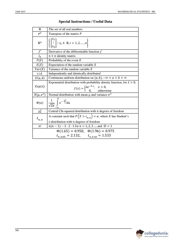
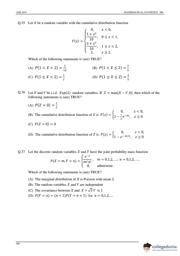
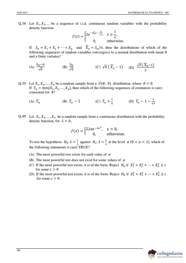
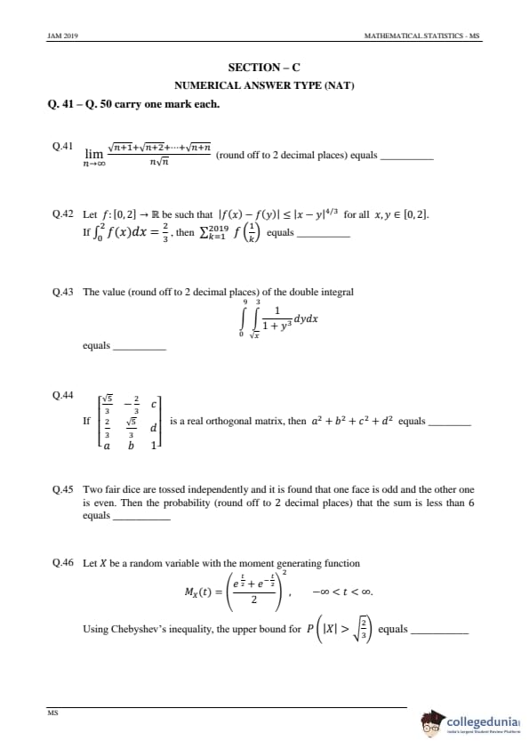
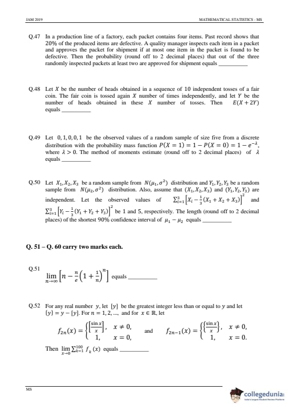

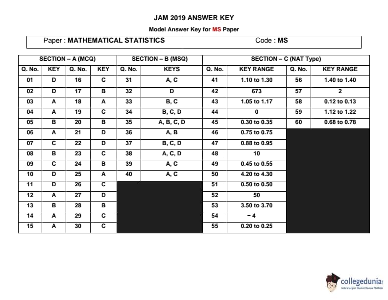
IIT JAM Previous Year Question Papers
| IIT JAM 2022 Question Papers | IIT JAM 2021 Question Papers | IIT JAM 2020 Question Papers |
| IIT JAM 2019 Question Papers | IIT JAM 2018 Question Papers | IIT JAM Practice Papers |
Comments