

.png?h=56&w=56&mode=stretch)


Karnataka PGCET 2026 Computer Science Engineering Question Paper is available for download here. Karnataka Examinations Authority (KEA) is conducting Karnataka PGCET 2026 CSE exam on May 23 in single shift from 2.30 pm to 4.30 pm. Karnataka PGCET 2026 CSE Question Paper consists of 100 questions for 100 marks to be attempted in 120 minutes.
- Karnataka PGCET 2026 Question Paper is divided into Engineering Mathematics, C Programming, Technical English and Engineering Domain questions.
- Each correct answer carries 1 mark and there is no negative marking for incorrect answers.
Karnataka PGCET 2026 CSE Question Paper with Solutions
| Karnataka PGCET CSE Question Paper 2026 | Download PDF | Check Solutions |
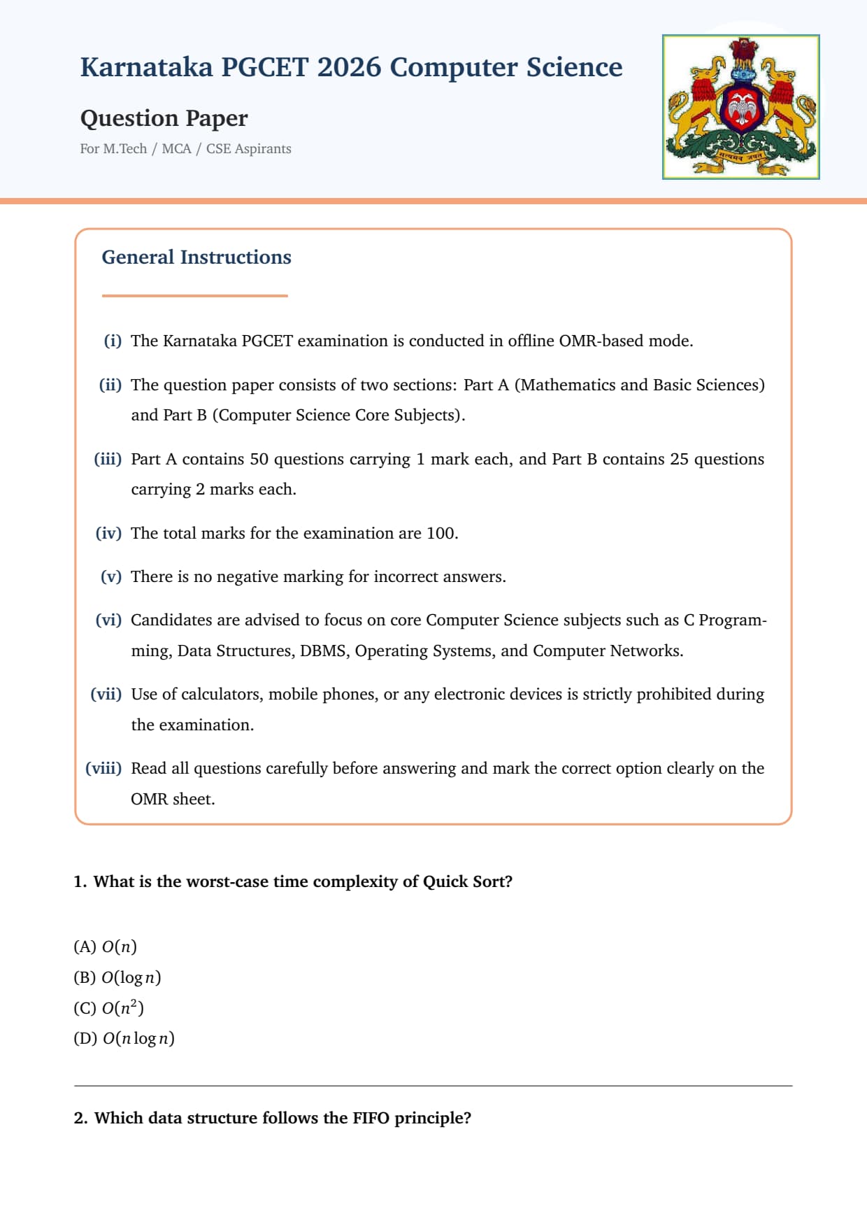
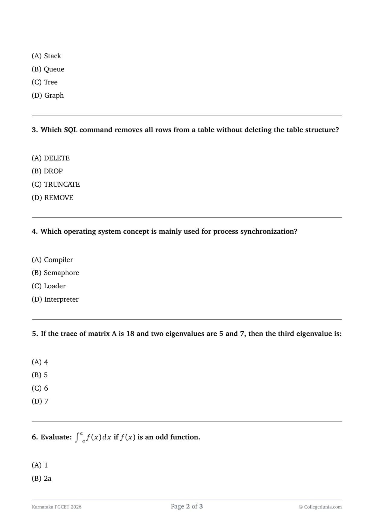
What is the worst-case time complexity of Quick Sort?
View Solution
Step 1: Understanding the Concept:
Quick Sort is a prominent sorting algorithm that utilizes the divide-and-conquer strategy to organize elements in an array.
The core idea is to select a 'pivot' element and partition the other elements into two sub-arrays according to whether they are less than or greater than the pivot.
The efficiency of this algorithm is heavily dependent on the choice of the pivot and the distribution of the data.
While it is famous for its \(O(n \log n)\) average-case performance, the worst-case scenario occurs when the partition is consistently unbalanced.
In such cases, the recursive structure of the algorithm fails to divide the problem into roughly equal halves, leading to degraded performance.
Step 2: Key Formula or Approach:
The time complexity of Quick Sort can be analyzed using a recurrence relation based on the partitioning logic.
For an array of size \(n\), let \(T(n)\) be the time taken to sort the array.
The partitioning step itself takes \(\theta(n)\) time because every element must be compared with the pivot once.
The recurrence is: \(T(n) = T(k) + T(n - k - 1) + \theta(n)\), where \(k\) is the number of elements smaller than the pivot.
In the worst-case scenario, the pivot is either the smallest or the largest element in the current sub-array at every step.
Step 3: Detailed Explanation:
Consider an input array that is already sorted in ascending order.
If the algorithm always selects the first element as the pivot, the partition will result in one sub-array of size \(0\) and another of size \(n-1\).
In the next recursive call, the sub-array of size \(n-1\) will again be split into \(0\) and \(n-2\).
This pattern continues until the size of the sub-array becomes \(1\).
The total time complexity is the sum of the work done at each level of recursion:
\[ T(n) = n + (n-1) + (n-2) + \dots + 1 \]
Mathematically, this is an arithmetic progression with a sum given by the formula:
\[ \sum_{i=1}^{n} i = \frac{n(n+1)}{2} \]
Expanding this gives \(\frac{1}{2}n^2 + \frac{1}{2}n\).
In Big O notation, we ignore lower-order terms and constants, resulting in \(O(n^2)\).
This quadratic complexity is significantly worse than the logarithmic depth seen in the best-case scenario.
To prevent this, modern implementations often use a "Randomized Quick Sort" where the pivot is chosen randomly.
Another common strategy is the "Median-of-Three" rule, where the pivot is selected as the median of the first, middle, and last elements.
These optimizations ensure that the probability of encountering the \(O(n^2)\) worst case is practically negligible in real-world scenarios.
Furthermore, when the recursion depth becomes too high, some hybrid algorithms like "Introsort" switch to Heap Sort to maintain a guaranteed \(O(n \log n)\) limit.
Step 4: Final Answer:
The worst-case time complexity of Quick Sort is \(O(n^2)\), which typically happens when the pivot consistently results in highly skewed partitions.
Quick Tip: Quick Sort is often preferred over Merge Sort due to lower constant factors and in-place sorting, but always be wary of the \(O(n^2)\) trap on pre-sorted data!
Which data structure follows the FIFO principle?
View Solution
Step 1: Understanding the Concept:
Data structures define how data is organized, managed, and stored to enable efficient access and modification.
Linear data structures like Stacks and Queues are defined by the specific order in which elements enter and leave the system.
FIFO stands for "First-In, First-Out."
This principle dictates that the first element added to the collection must be the first one to be removed.
This is similar to a queue of people at a ticket counter: the person who arrives first is served first.
Step 2: Detailed Explanation:
Let's analyze the fundamental behavior of the structures provided in the options.
1. Stack: Operates on the LIFO (Last-In, First-Out) principle. Elements are pushed and popped from the same end (the top). Example: a stack of plates.
2. Queue: Operates on the FIFO principle. It has two distinct ends: the 'Front' for removal and the 'Rear' for insertion.
3. Tree: A hierarchical, non-linear data structure. It does not follow a strict temporal order like FIFO; instead, it represents parent-child relationships.
4. Graph: A complex non-linear structure consisting of vertices and edges. While traversals like BFS use a queue, the graph itself isn't a FIFO structure.
In a standard Queue, there are two primary operations: Enqueue and \textit{Dequeue.
When you \textit{Enqueue an item, it is placed at the back of the line.
When you \textit{Dequeue an item, the item currently at the front is removed.
This ensures that the processing order is strictly sequential based on arrival time.
Step 3: Detailed Explanation:
Consider an sequence of inputs: [A, B, C].
In a Queue:
- Enqueue A \(\to\) [A]
- Enqueue B \(\to\) [A, B]
- Enqueue C \(\to\) [A, B, C]
- Dequeue \(\to\) Returns A (The first one that entered).
Contrast this with a Stack:
- Push A \(\to\) [A]
- Push B \(\to\) [A, B]
- Push C \(\to\) [A, B, C]
- Pop \(\to\) Returns C (The last one that entered).
Queues are essential in computer science for scenarios where resources are shared among multiple consumers.
Examples include CPU task scheduling (Ready Queue), IO buffers, and printer spoolers.
Advanced variations include the "Circular Queue" to optimize memory usage and "Priority Queues" where FIFO is modified by urgency.
However, the base implementation of a linear queue is the definitive example of the FIFO principle.
Step 4: Final Answer:
The Queue is the data structure that strictly follows the FIFO (First-In, First-Out) principle.
Quick Tip: Remember \textbf{FIFO = Queue (like a line for coffee) and \textbf{LIFO = Stack} (like a stack of books). This distinction is fundamental for almost every technical interview!
Which SQL command removes all rows from a table without deleting the table structure?
View Solution
Step 1: Understanding the Concept:
In Database Management Systems (DBMS), we often need to manage the lifecycle of data within tables.
Sometimes we need to clear out all the records in a table to start fresh, while keeping the container (the table definition) ready for new entries.
SQL provides several commands that might seem similar but have distinct impacts on the database schema and logging mechanisms.
The main choices are DELETE, DROP, and TRUNCATE.
Step 2: Detailed Explanation:
Let's break down the mechanics of the options provided:
1. DELETE: This is a Data Manipulation Language (DML) command. It scans the table and deletes rows one by one. Because it logs every single row deletion, it is relatively slow for large datasets. You can use a \texttt{WHERE clause to target specific rows. Crucially, it does not reset the table's identity/auto-increment seed.
2. DROP: This is a Data Definition Language (DDL) command. It removes the entire table object from the database metadata. The data, the structure, the indexes, and the constraints are all gone. You cannot insert data into a dropped table without a \texttt{CREATE TABLE statement.
3. TRUNCATE: This is also a DDL command. It is designed to "wipe" the table clean. It doesn't scan rows; instead, it deallocates the data pages that store the records. This makes it incredibly fast. It preserves the structure, constraints, and indexes but removes all data and resets any auto-increment counters to their original starting point.
4. REMOVE: This is not a standard SQL command. While some specific non-SQL systems might use it, it is not part of standard ANSI SQL for table management.
Step 3: Detailed Explanation:
The choice between DELETE and TRUNCATE usually depends on the use case.
If you need to maintain a transaction log for each row (for auditing or partial rollbacks), use DELETE.
If you are clearing a temporary table or an staging area and want maximum performance, TRUNCATE is the best choice.
However, TRUNCATE has limitations:
- It cannot be used on a table that is referenced by a Foreign Key constraint.
- It is considered a DDL operation, so in some databases (like Oracle), it implicitly commits the current transaction.
- Because it is a "bulk" operation, it typically generates less redo and undo log space than a DELETE statement of equal volume.
In summary, because the question asks to remove all rows while preserving the structure, TRUNCATE is the most efficient and accurate answer.
Step 4: Final Answer:
The TRUNCATE command is the correct SQL instruction for removing all records while keeping the table structure intact.
Quick Tip: If you want to keep the "container" but empty the "contents" fast, use \textbf{TRUNCATE}. If you want to throw the "container" away entirely, use \textbf{DROP}.
Which operating system concept is mainly used for process synchronization?
View Solution
Step 1: Understanding the Concept:
In a concurrent computing environment, multiple processes or threads often share the same hardware and software resources.
When these processes access shared data simultaneously, they can interfere with each other, leading to inconsistent or corrupted data—a situation known as a "Race Condition."
Process synchronization is the set of techniques used to ensure that only one process can access a critical section of code at a time.
Without proper synchronization, even simple operations like incrementing a shared counter can fail if two processes attempt it at the exact same moment.
Step 2: Detailed Explanation:
Let's evaluate the options to identify the one related to OS process management:
1. Compiler: A system program that converts high-level code to machine code. It does not handle runtime execution synchronization.
2. Semaphore: A variable or abstract data type used to control access to a common resource by multiple processes. It is a fundamental synchronization primitive.
3. Loader: Responsible for loading the executable code into memory before a process starts. It is not involved in coordinating concurrent processes during execution.
4. Interpreter: Executes code line-by-line without prior compilation. Like the compiler, it's a language tool, not a synchronization mechanism.
Step 3: Detailed Explanation:
A Semaphore, introduced by Edsger Dijkstra, is essentially an integer counter that processes use to communicate about resource availability.
There are two main types of Semaphores:
- Binary Semaphore (Mutex): Can only have values 0 or 1. It acts as a lock. If the value is 1, a process can take the lock (set it to 0) and proceed. Others must wait until the lock is released.
- Counting Semaphore: Its value can represent the total number of available instances of a resource (e.g., a pool of 5 network connections).
The operations on a semaphore are atomic, meaning they cannot be interrupted. These are:
- Wait (P operation): Decrements the semaphore value. If the resulting value is negative, the process is blocked and added to a waiting queue.
- Signal (V operation): Increments the semaphore value. If there are processes waiting, one is unblocked and allowed to proceed.
By carefully placing these operations around "Critical Sections," the OS ensures that data integrity is maintained across all running threads.
Step 4: Final Answer:
The Semaphore is the primary mechanism among the options used for process synchronization in operating systems.
Quick Tip: Semaphores help solve the "Producer-Consumer" and "Dining Philosophers" problems. Think of a semaphore as a key to a room; if the key is taken, you must wait outside!
If the trace of matrix A is 18 and two eigenvalues are 5 and 7, then the third eigenvalue is:
View Solution
Step 1: Understanding the Concept:
In Linear Algebra, the properties of square matrices are often analyzed through their eigenvalues.
An eigenvalue \(\lambda\) of a matrix \(A\) is a scalar that satisfies the equation \(Av = \lambda v\) for some non-zero vector \(v\).
One of the most important theorems regarding eigenvalues relates them to the "Trace" of the matrix.
The Trace, denoted as \(Tr(A)\), is simply the sum of the elements on the main diagonal of the matrix.
Step 2: Key Formula or Approach:
The fundamental property used here is:
The sum of all eigenvalues of a square matrix is equal to the trace of that matrix.
If a matrix \(A\) is of size \(n \times n\), it has exactly \(n\) eigenvalues (counting multiplicity).
The formula is:
\[ \sum_{i=1}^{n} \lambda_i = Tr(A) \]
Step 3: Detailed Explanation:
From the problem description, we can infer that the matrix is likely a \(3 \times 3\) matrix because three eigenvalues are discussed.
We are given the following data points:
- Trace of matrix \(A = 18\).
- First eigenvalue, \(\lambda_1 = 5\).
- Second eigenvalue, \(\lambda_2 = 7\).
- Let the third eigenvalue be \(\lambda_3\).
Using the trace property formula:
\[ \lambda_1 + \lambda_2 + \lambda_3 = Tr(A) \]
Plugging in the numerical values provided:
\[ 5 + 7 + \lambda_3 = 18 \]
Combine the known numbers:
\[ 12 + \lambda_3 = 18 \]
To find the unknown eigenvalue \(\lambda_3\), subtract 12 from both sides of the equation:
\[ \lambda_3 = 18 - 12 \]
\[ \lambda_3 = 6 \]
This relationship is derived from the fact that the trace of a matrix is invariant under similarity transformations, and the diagonal form of a matrix (if it exists) has the eigenvalues on its diagonal.
Similarly, the product of the eigenvalues is equal to the determinant of the matrix, which is another useful property for solving matrix-related problems.
Step 4: Final Answer:
The value of the third eigenvalue is 6.
Quick Tip: For Eigenvalues:
\textbf{Sum = Trace}
\textbf{Product = Determinant}
Memorizing these two facts will allow you to solve almost any MCQ on eigenvalue properties in seconds!
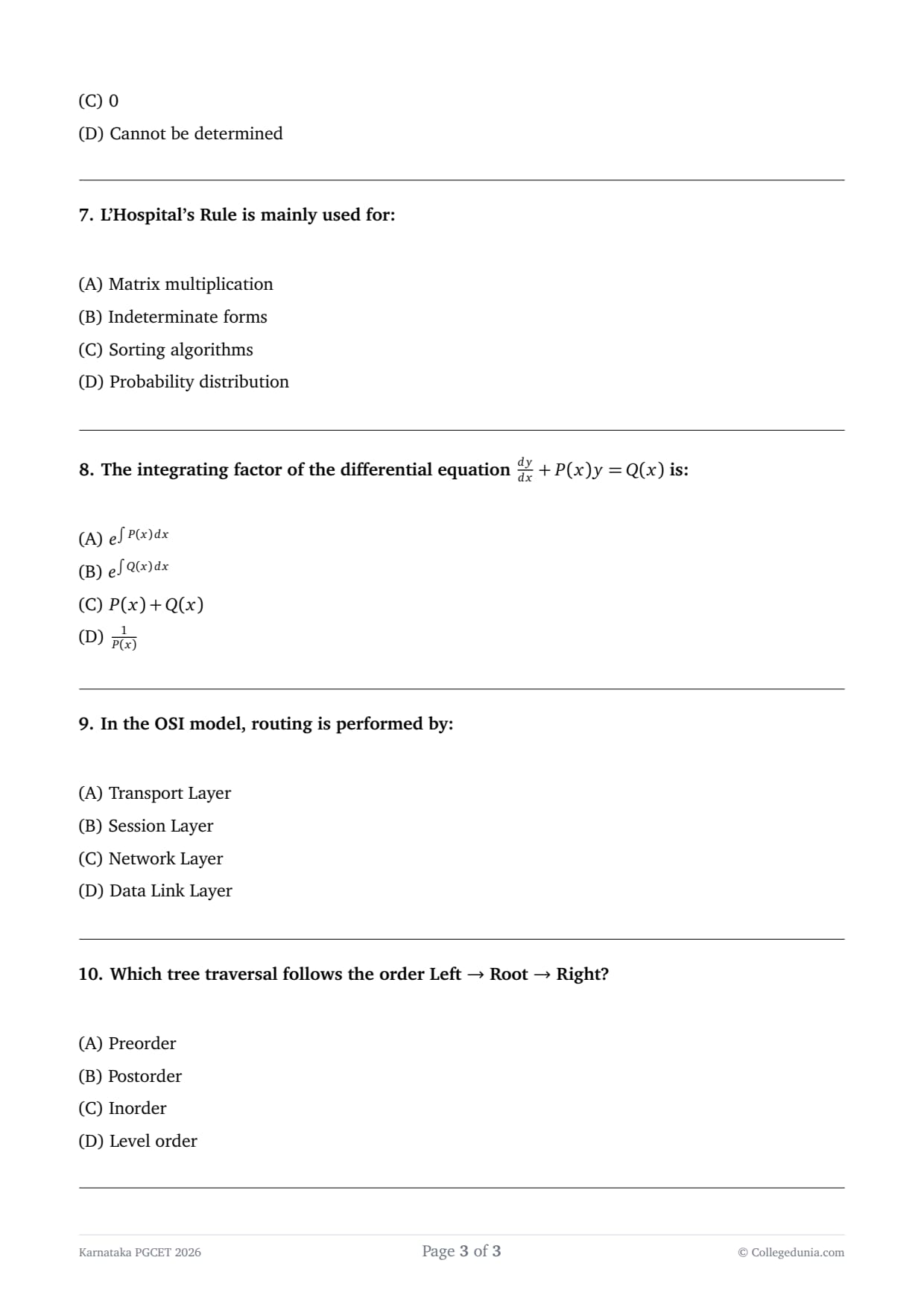
Evaluate: \( \int_{-a}^{a} f(x) \, dx \) if \(f(x)\) is an odd function.
View Solution
Step 1: Understanding the Concept:
In calculus, we can simplify the evaluation of definite integrals by identifying the symmetry of the integrand.
A function \(f(x)\) is called an "odd function" if it satisfies the mathematical condition \(f(-x) = -f(x)\) for all \(x\) in its domain.
Graphically, an odd function is symmetric with respect to the origin. Examples include \(\sin(x)\), \(x^3\), and \(x\).
When we integrate a function over a symmetric interval \([-a, a]\), we are calculating the signed area between the curve and the x-axis from \(-a\) to \(a\).
Step 2: Key Formula or Approach:
The general property for integrals with symmetric limits is:
- If \(f(x)\) is even (\(f(-x) = f(x)\)), then \(\int_{-a}^{a} f(x) \, dx = 2 \int_{0}^{a} f(x) \, dx\).
- If \(f(x)\) is odd (\(f(-x) = -f(x)\)), then \(\int_{-a}^{a} f(x) \, dx = 0\).
Step 3: Detailed Explanation:
Let's prove why the integral of an odd function over symmetric limits is zero.
We can split the integral at the origin:
\[ \int_{-a}^{a} f(x) \, dx = \int_{-a}^{0} f(x) \, dx + \int_{0}^{a} f(x) \, dx \]
Focusing on the first integral, let's use the substitution \(x = -t\), which implies \(dx = -dt\).
When \(x = -a\), \(t = a\). When \(x = 0\), \(t = 0\).
The integral becomes:
\[ \int_{a}^{0} f(-t) (-dt) = \int_{0}^{a} f(-t) \, dt \]
Since \(f(x)\) is an odd function, we know \(f(-t) = -f(t)\).
Substituting this back:
\[ \int_{0}^{a} -f(t) \, dt = -\int_{0}^{a} f(t) \, dt \]
Now, combining this result back into our original split integral:
\[ \int_{-a}^{a} f(x) \, dx = -\int_{0}^{a} f(t) \, dt + \int_{0}^{a} f(x) \, dx \]
Since the variable name in a definite integral is irrelevant (dummy variable), \(\int_{0}^{a} f(t) \, dt = \int_{0}^{a} f(x) \, dx\).
The terms cancel out: \( -K + K = 0 \).
Geometrically, the area to the left of the y-axis is below the x-axis and the area to the right is above (or vice versa), and because they are identical in size but opposite in sign, they sum to exactly zero.
Step 4: Final Answer:
The integral evaluate to 0 because the function is odd and the limits are symmetric.
Quick Tip: Always check the limits first. If you see \(\int_{-a}^{a}\), look for whether the function is odd. If it is, don't bother calculating; the answer is \textbf{0}!
L'Hospital's Rule is mainly used for:
View Solution
Step 1: Understanding the Concept:
When calculating limits in calculus, we frequently encounter cases where substituting the target value directly into a quotient results in an undefined expression.
Specifically, if we have \(\lim_{x \to c} \frac{f(x)}{g(x)}\) and both functions approach 0 or both approach infinity, we get expressions like \(\frac{0}{0}\) or \(\frac{\infty}{\infty}\).
These are called "Indeterminate Forms" because the value of the limit is not obvious and could be anything (or not exist at all).
L'Hospital's Rule provides a powerful method to resolve these ambiguities using differentiation.
Step 2: Key Formula or Approach:
The rule states that if the limit of \(\frac{f(x)}{g(x)}\) as \(x\) approaches \(c\) results in an indeterminate form, then:
\[ \lim_{x \to c} \frac{f(x)}{g(x)} = \lim_{x \to c} \frac{f'(x)}{g'(x)} \]
This holds true as long as the limit on the right exists and \(g'(x)\) is non-zero near \(c\).
Step 3: Detailed Explanation:
There are several types of indeterminate forms where L'Hospital's Rule or its variants can be applied:
1. Primary forms: \(\frac{0}{0}\) and \(\frac{\infty}{\infty}\). These are the direct applications for the rule.
2. Product forms: \(0 \cdot \infty\). These are solved by rewriting the product as a quotient, e.g., \(f \cdot g = \frac{f}{1/g}\), creating a \(\frac{0}{0}\) or \(\frac{\infty}{\infty}\) scenario.
3. Difference forms: \(\infty - \infty\). These usually require finding a common denominator to turn the expression into a fraction.
4. Power forms: \(1^{\infty}, 0^0, \infty^0\). These are handled by taking the natural logarithm (\(\ln\)) of the expression, solving the limit, and then exponentiating back.
L'Hospital's rule is fundamentally a statement about local linearity. Near the point \(c\), the functions behave like their tangent lines. The ratio of the functions is thus effectively the ratio of their slopes (derivatives).
It is important to remember not to use the quotient rule when applying L'Hospital's; instead, you differentiate the numerator and denominator independently.
Step 4: Final Answer:
L'Hospital's Rule is the standard tool for evaluating limits that result in indeterminate forms.
Quick Tip: Before applying L'Hospital's Rule, \textbf{always verify} that you have \(0/0\) or \(\infty/\infty\). If you apply it to a regular limit like \(5/2\), you will get the wrong answer!
The integrating factor of the differential equation \( \frac{dy}{dx} + P(x)y = Q(x) \) is:
View Solution
Step 1: Understanding the Concept:
A First-Order Linear Ordinary Differential Equation (ODE) is one that can be written in the standard form:
\[ \frac{dy}{dx} + P(x)y = Q(x) \]
The difficulty in solving this directly is that the left side isn't a perfect derivative of any single expression.
The technique of the "Integrating Factor" involves finding a special function, let's call it \(M(x)\), that we can multiply across the whole equation to make the left side a derivative of a product.
This transformation allows us to integrate directly and solve for \(y\).
Step 2: Key Formula or Approach:
The standard formula for the Integrating Factor (IF) is:
\[ IF = e^{\int P(x) \, dx} \]
Step 3: Detailed Explanation:
Let's see how this works. We want to find a function \(M(x)\) such that:
\[ M(x) \left[ \frac{dy}{dx} + P(x)y \right] = \frac{d}{dx} [M(x)y] \]
Using the product rule on the right side:
\[ M(x) \frac{dy}{dx} + M(x)P(x)y = M(x) \frac{dy}{dx} + y \frac{dM}{dx} \]
Comparing the terms, we must have:
\[ M(x)P(x) = \frac{dM}{dx} \]
This is a separable differential equation for \(M(x)\):
\[ \frac{dM}{M} = P(x) \, dx \]
Integrating both sides gives:
\[ \ln |M| = \int P(x) \, dx \]
Exponentiating both sides results in:
\[ M(x) = e^{\int P(x) \, dx} \]
Once the differential equation is multiplied by this factor, it becomes:
\[ \frac{d}{dx} [y \cdot e^{\int P(x) \, dx}] = Q(x) \cdot e^{\int P(x) \, dx} \]
The general solution is then found by integrating both sides with respect to \(x\):
\[ y \cdot IF = \int (Q(x) \cdot IF) \, dx + C \]
This method is incredibly efficient for linear first-order equations and is a staple in engineering and physics problem-solving.
Step 4: Final Answer:
The integrating factor for the given standard linear ODE is \( e^{\int P(x) \, dx} \).
Quick Tip: Before finding \(P(x)\), make sure the coefficient of \(\frac{dy}{dx}\) is exactly \textbf{1}. If you have \(x \frac{dy}{dx} + 2y = \dots\), divide the whole equation by \(x\) first!
In the OSI model, routing is performed by:
View Solution
Step 1: Understanding the Concept:
The Open Systems Interconnection (OSI) model is a conceptual framework developed by the International Organization for Standardization (ISO).
It partitions a communication system into seven abstraction layers, which are (from bottom to top): Physical, Data Link, Network, Transport, Session, Presentation, and Application.
Each layer has a specific set of duties and protocols that allow disparate systems to communicate over a network.
Routing is the fundamental process of moving data packets from a source host to a destination host across multiple interconnected networks.
Step 2: Detailed Explanation:
To answer this, let's examine the primary functions of the relevant layers:
1. Data Link Layer (Layer 2): Handles node-to-node data transfer—between two directly connected nodes. It uses MAC (Media Access Control) addresses. It doesn't know about the larger network "path."
2. Network Layer (Layer 3): This is the layer responsible for "logical addressing" and "path determination." It manages IP addresses and decides the best physical path for the data based on network conditions and priorities. This is exactly where routing occurs.
3. Transport Layer (Layer 4): Provides transparent transfer of data between end users, providing reliable data transfer services. It manages end-to-end communication (using ports), not the route taken through the intermediate nodes.
4. Session Layer (Layer 5): Controls the dialogues (connections) between computers. It establishes, manages, and terminates connections between local and remote applications.
Step 3: Detailed Explanation:
The device associated with the Network Layer is the Router.
A router maintains a routing table that maps destination network prefixes to the "Next Hop" (the next router in the chain).
When a packet arrives, the Network Layer logic extracts the destination IP address, searches the routing table for the most specific match, and forwards the packet out of the corresponding interface.
Protocols like IP (Internet Protocol), ICMP, OSPF, and BGP all operate at this layer to ensure that data can find its way across the global internet.
Without Layer 3, we would only be able to communicate with devices on our local physical segment.
Therefore, the Network Layer is the "traffic controller" of the OSI model.
Step 4: Final Answer:
In the OSI model, routing is the core responsibility of the Network Layer.
Quick Tip: Layer 2 (Data Link) = Switches \& MAC Addresses.
Layer 3 (Network) = \textbf{Routers} \& IP Addresses.
Routing and IP always go together in Layer 3!
Which tree traversal follows the order Left \(\to\) Root \(\to\) Right?
View Solution
Step 1: Understanding the Concept:
Tree traversal is the algorithmic process of visiting (checking or updating) each node in a tree data structure exactly once.
For binary trees, the most common traversals are recursive and fall under the "Depth-First Search" (DFS) category.
These traversals are defined by the relative order in which we visit the root node compared to its left and right subtrees.
Step 2: Detailed Explanation:
Let's define the sequence for each common traversal type:
1. Preorder Traversal: Root \(\to\) Left \(\to\) Right. The root is processed first. Useful for creating a copy of the tree or evaluating prefix expressions.
2. Inorder Traversal: Left \(\to\) Root \(\to\) Right. The root is processed in between its subtrees. This is the sequence specified in the question.
3. Postorder Traversal: Left \(\to\) Right \(\to\) Root. The root is processed last. Useful for deleting a tree or evaluating postfix expressions.
4. Level Order Traversal: Processes nodes level-by-level from top to bottom. This is a Breadth-First Search (BFS) technique.
Step 3: Detailed Explanation:
Inorder traversal has a very special property in the context of Binary Search Trees (BSTs).
In a BST, all values in the left subtree are smaller than the root, and all values in the right subtree are larger.
Because Inorder visits "Smaller elements (Left) \(\to\) Current element (Root) \(\to\) Larger elements (Right)", performing an Inorder traversal on a BST will visit the nodes in perfectly sorted (ascending) order.
Example: Consider a tree with 5 as Root, 3 as Left child, and 7 as Right child.
- Preorder: 5, 3, 7
- Inorder: 3, 5, 7
- Postorder: 3, 7, 5
The request "Left \(\to\) Root \(\to\) Right" is the textbook definition of the Inorder sequence.
Implementation is typically done via recursion where the function calls itself on the left child, prints the current node value, and then calls itself on the right child.
Step 4: Final Answer:
The tree traversal order that visits nodes in the sequence Left \(\to\) Root \(\to\) Right is Inorder traversal.
Quick Tip: To remember easily:
\textbf{Pre} means root \textbf{before} children.
\textbf{In} means root \textbf{between} children.
\textbf{Post} means root \textbf{after} children.
Karnataka PGCET 2026 Exam Pattern
| Parameter | Details |
|---|---|
| Exam Mode | OMR based |
| Exam Duration | 120 minutes |
| Question Type | Multiple Choice Questions (MCQs) |
| Total Questions | 100 questions (all compulsory) |
| Maximum Marks | 100 |
| Marking Scheme | +1 for correct, 0 for incorrect |



Comments