These Electrostatic Potential and Capacitance Class 12 Physics Chapter 2 Exemplar Solutions solve all 33 problems, each with a clean Solution and an Expert's Solution. They cover capacitors, dielectrics, equipotentials and ring potentials, aligned to the 2026-27 NCERT syllabus. You can read every answer here and download the PDF on this page.
33 problems split across 6 MCQ-I, 7 MCQ-II, 5 VSA, 5 SA and 10 LA
Two-tab format: short Solution + expanded Expert's Solution per question, mapped to the last five years of JEE Main, JEE Advanced and NEET PYQs
Free PDF, printable in A4, refreshed for 2026-27
33 Exemplar problems · 6 MCQ-I + 7 MCQ-II + 5 VSA + 5 SA + 10 LA · Class 12 Physics Chapter 2, 2026-27 NCERT
CBSE Weightage: 6 to 8 marks (a short answer plus one numerical or 5-mark derivation)
JEE Main Weightage: 3 to 4% (about 1 question per shift, mostly dielectric and combination)
NEET Weightage: 1 to 2 questions per year
The PDF below works on phone and desktop, and you can flip through it in the reader. Every problem is solved twice: a short Solution and a longer Expert's Solution.
This set is built by subject experts, mapped to the 2026-27 NCERT, and checked against the last five years of CBSE Board, JEE Main and NEET papers.
Electrostatic Potential and Capacitance Exemplar: MCQ, VSA, SA and LA Counts at a Glance
Chapter 2 leans on Long Answer items more than any other chapter in the Electrostatics unit. The 10 LA problems carry the most reused JEE and NEET setups, and the 7 MCQ-II items hide double-correct traps on dielectrics.
Question Type
Range
Count
Marks
Total Time
MCQ-I (single-correct)
2.1 to 2.6
6
1
15 min
MCQ-II (multiple-correct)
2.7 to 2.13
7
2
30 min
VSA (very short)
2.14 to 2.18
5
1 to 2
20 min
SA (short answer)
2.19 to 2.23
5
3
40 min
LA (long answer)
2.24 to 2.33
10
5
110 min
Quick Tip: Treat the 10 LA items (2.24 to 2.33) as your main JEE Advanced and CBSE 5-marker practice set. They cover ring and disc potentials, dielectrics and the disc-lifting numerical.
Electrostatic Potential and Capacitance NCERT Exemplar Video Solutions
The quickest way to crack the capacitor problems here is simple. First tag whether the battery is on (V fixed) or off (Q fixed), then read off C, E and U. The full step-by-step set for all 33 problems sits in the cards lower down.
Why Use this NCERT Exemplar Class 12 Physics for Board, JEE and NEET?
Each problem carries a clean Solution plus an Expert's Solution that names every concept used.
Every type solved: all 6 MCQ-I, 7 MCQ-II, 5 VSA, 5 SA and 10 LA, with full reasoning.
Concept named in each step: equipotential property, clamp logic, dielectric energy, or surface-charge scaling.
JEE and NEET bridge: items 2.1, 2.13, 2.20 and 2.30 are tagged with the year an entrance exam reused them.
Electrostatic Potential and Capacitance Weightage Across Class 12 Physics Chapters
Chapter 2 is the heaviest LA-loaded chapter in the syllabus, worth a steady 4 to 7 marks in CBSE board years. The table below puts it next to the other chapters so students can plan revision time.
Chapter
Topic
Avg CBSE Marks
Ch 1
Electric Charges and Fields
4 marks
Ch 2
Electrostatic Potential and Capacitance
4 to 7 marks
Ch 3
Current Electricity
7 marks
Ch 4
Moving Charges and Magnetism
5 marks
Ch 5
Magnetism and Matter
3 marks
Ch 6
Electromagnetic Induction
5 marks
Ch 7
Alternating Current
3 marks
Ch 8
Electromagnetic Waves
2 marks
Ch 9
Ray Optics and Optical Instruments
5 marks
Ch 10
Wave Optics
5 marks
Ch 11
Dual Nature of Radiation and Matter
4 marks
Ch 12
Atoms
3 marks
Ch 13
Nuclei
3 marks
Ch 14
Semiconductor Electronics
7 marks
Chapter 2 often pairs with Chapter 1 in CBSE Section-D 5-markers, so revise both together. It also shows up in JEE Main shift papers about once per session.
Electrostatic Potential and Capacitance Class 12th: Difficulty Step-Up from NCERT Textbook to Exemplar
The textbook tests one dielectric slab at a time. The Exemplar chains two or three ideas per problem and sets traps the textbook never does.
Concept
NCERT Textbook Setup
Exemplar Twist
Capacitor with battery
Direct Q = CE on an ideal battery
2.1: add internal resistance, so only the terminal voltage drives the capacitor
Series dielectrics
One slab between plates
2.6: two dielectrics in series, derive the harmonic-mean k
Disconnect-and-modify
One variable changes
2.20: track all of C, V, E, Q, U when the slab is pulled out
Surface charge density
Single sphere
2.30: two spheres of different R touch, then separate, so σ redistributes
Potential function
Point charge at a fixed point
2.17: prove no max or min can exist in free space (Laplace's equation)
Exemplar-Specific Common Mistakes in Electrostatic Potential and Capacitance
These slips show up once Exemplar's chained logic kicks in.
Using EMF instead of terminal voltage across the capacitor in 2.1. This is JEE Main's standard 4-mark trap.
Forgetting V is clamped but Q is not when the battery stays on in 2.13.
Treating σ as constant on contact in 2.30. Spheres equalise potentials, not charge densities.
Quoting disc potential as ring potential in 2.32 vs 2.33.
Skipping the unstable-equilibrium check in 2.24 and 2.33, which the 5-mark scheme needs.
Electrostatic Potential and Capacitance Top 5 Formulae for Exemplar Numericals
These five formulae carry most of the SA and LA load.
Quantity
Formula
Potential of a point charge
V = 14π0 · qr
Potential on the axis of a ring
( V(z) = 14π0 · Q√z2 + R2} )
Parallel-plate capacitance
C = 0A / d (vacuum) C = k0A / d (dielectric)
Energy stored in a capacitor
U = 12 CV2 = Q22C = 12 QV
Series and parallel combination
Series: 1/Cs = ∑ 1/Ci
Parallel: Cp = ∑ Ci
Class 12 Physics NCERT Exemplar PDF for Electrostatic Potential and Capacitance: Editions and Format
The Chapter 2 Exemplar PDF above is free and works on phone and desktop. It comes in a few formats.
Standard and HD page resolutions, with a separate HD download link.
Hindi-medium edition for students who study Physics in Hindi.
An MCQ-only sub-set (MCQ-I plus MCQ-II) inside the same file for quick revision.
The page solves the problems in the same order as the printed book, so students can cross-check side by side. For more practice, pair it with the NCERT Solutions for Chapter 2.
All NCERT Exemplar Questions for Electrostatic Potential and Capacitance with Step-by-Step Solutions
Every question of the NCERT Exemplar set for Class 12 Physics Chapter 2 Electrostatic Potential and Capacitance is listed below with its full Solution and Expert Solution hidden inside collapsible tabs. Click Check Solution to reveal the step-by-step working; click Expert Solution for the expanded explanation.
MCQ I (single correct option)
Q 2.1
A 4 capacitor is connected as shown in Fig. 2.1. The internal resistance of the battery is 0.5 Ω. The charge on the capacitor plates will be:
(a) 0 (b) 4 (c) 16 (d) 8 .
Concept used. In the steady state of a DC circuit
containing a capacitor, no current flows through the capacitor
branch, because once the capacitor is fully charged, the displacement
of charge stops. The voltage across a capacitor in steady state
equals the potential difference between its terminals as fixed by
the rest of the circuit.
Capacitor in steady DC
A capacitor in steady state behaves like an open circuit. Any
resistor in series with it carries zero current, hence zero IR drop.
The voltage across the capacitor equals the voltage across whatever
parallel branch sits between the same two nodes.
Identify the conducting branch. The capacitor
(4 ) sits in series with the 10 Ω
resistor in the upper branch. The lower branch contains the
2 Ω resistor. Both branches are in parallel across
the battery (EMF E = 2.5 V, internal resistance
r = 0.5 Ω). In steady state, no current passes
through the upper branch (capacitor blocks DC), so the only
loop carrying current is: battery →2 Ω→
battery.
Find the current. Apply Kirchhoff's voltage law to
the loop battery + r + 2 Ω:
E = I (r + R),
where R = 2 Ω is the load and r = 0.5 Ω is
the internal resistance. Substitute:
2.5 = I (0.5 + 2) = 2.5 II = 1 A.
Find the terminal voltage of the battery. This is
also the potential difference across the parallel external
load:
Vterm = E - Ir = 2.5 - (1)(0.5) = 2.0 V.
Equivalently, Vterm = IR = (1)(2) = 2.0 V across the
2 Ω. Either route gives the same number.
Find the voltage across the capacitor. Since no
current flows through the upper branch, the IR drop across
the 10 Ω resistor is
V10Ω = (0)(10) = 0 V.
The whole terminal voltage therefore appears across the
capacitor:
VC = Vterm - V10Ω = 2.0 - 0 = 2.0 V.
Compute the charge. Use Q = C VC:
Q = (4 )(2 V) = 8 .
Sanity check
The answer must be ≤ C · E = (4)(2.5) = 10 μC
(the absolute upper bound on a 4 μF capacitor across a 2.5 V
source). Our 8 μC is comfortably under this ceiling.
Q = 8 (Option (d))
AI
Aarav Iyer
M.Sc Physics, IIT Madras
Verified Expert
Strategic angle. The branch-by-branch approach is most
foolproof here: spot which loop actually carries current, get the
common terminal voltage, then read the capacitor voltage off the
upper branch.
Why the upper branch is dead. A capacitor in steady
state stores charge and rejects further current. So
Iupper = 0, and the 10 Ω resistor
contributes no voltage drop.
Lower-branch current. The only conducting loop is
battery → r → 2 Ω → battery. Ohm's law for
this loop:
I = Er + R = 2.5 V0.5 Ω + 2 Ω = 1 A.
Terminal voltage = voltage across capacitor. Both
branches share the same two end-nodes (the battery
terminals), so the voltage across the upper branch equals
that across the lower branch:
VC + V10Ω = V2Ω ⇒ VC + 0 = (1)(2) = 2 V.
The choice 10 μC is the deliberate trap: it forgets the
internal-resistance drop. Treating E = 2.5 V as the
voltage across the capacitor (instead of the terminal voltage
E - Ir) gives Q = 4 × 2.5 V = 10 μC, which is option (b) and the standard mistake.
Alternative method, Kirchhoff's voltage law explicitly.
Write KVL around the conducting loop (E → r → 2 Ω → back):
E - Ir - I(2 Ω) = 0 ⇒ I = 2.52.5 = 1 A.
Now traverse from one capacitor plate to the other via the lower
branch: starting at the top node, drop VC across C, then 0
across the 10 Ω resistor (no current), then -IR across
2 Ω, finishing at the bottom node. Since both branches share
the same end-nodes, the algebraic sum across each must match the
terminal voltage E - Ir = 2.5 - 0.5 = 2 V. Hence VC = 2 V.
Concept linkage. This problem stitches together Chapter 3
(current electricity and EMF with internal resistance) with the
chapter-2 capacitor relation Q = CV. Whenever a capacitor sits
in a branch with no other DC path, that branch carries zero
steady current, so all the voltage of the parallel branch piles
across the capacitor (resistors in that dead branch drop 0).
Exam tip. In CBSE board problems, this kind of
``capacitor-in-a-DC-circuit'' problem is a 2-mark or 3-mark
favourite. Show: (i) the steady-state current path; (ii) the
terminal/Branch voltage calculation; (iii) Q = CV. Skipping any
of these three steps usually costs the full mark for that step.
Q = 8 , option (d).
Q 2.2
A positively charged particle is released from rest in a uniform electric field. The electric potential energy of the charge:
(a) remains constant because the field is uniform.
(b) increases because the charge moves along the field.
(c) decreases because the charge moves along the field.
(d) decreases because the charge moves opposite to the field.
Concept used. A positive charge in an electric field
experiences a force in the direction of E⃗:
F⃗ = qE⃗. Starting from rest, it accelerates along
E⃗. The relation between work done by the electric force
and the change in electrostatic potential energy is
Welec = -Δ U = q(Vi - Vf).
Since the force does positive work on the charge, the change in
potential energy Δ U is negative, i.e. U decreases.
The lost potential energy reappears as kinetic energy.
Direction of E⃗ and V
E⃗ points from high V to low V. A positive charge,
following E⃗, moves from a high-potential region to a
low-potential region, so its PE U = qV decreases.
Direction of motion. Released from rest, the
particle accelerates in the direction of F⃗ = qE⃗.
Because q > 0, the motion is alongE⃗.
Potential change. Along the field, the potential
decreases:
Vf < Vi.
Potential-energy change.U = qV with q > 0, so
Δ U = q(Vf - Vi) < 0.
The PE decreases.
Energy conservation check. Since total mechanical
energy is conserved (no friction here), the lost PE shows
up as kinetic energy:
12m v2 = -Δ U > 0,
consistent with the particle speeding up.
PE decreases because the charge moves along the field. Option (c).
SK
Sneha Kapoor
M.Sc Physics, IIT Bombay
Verified Expert
Quick reading. Three facts decide this question:
F⃗ = qE⃗, the field points from higher to lower
potential, and U = qV for a point charge in an external field.
For q > 0, F⃗ is parallel to E⃗, so the
particle's displacement is along E⃗.
Moving along E⃗ takes the particle to lower potential.
Quantitatively, Vf - Vi = -ifE⃗· dl⃗ < 0.
Therefore Δ U = q Δ V < 0. The PE decreases.
This rules out (a), (b), (d). Option (d) is wrong because
a positive charge does not move opposite to E⃗
when released from rest; that would happen for a negative
charge.
Alternative method, energy conservation. No friction
acts, so mechanical energy is conserved: Ki + Ui = Kf + Uf.
With Ki = 0 (released from rest) and Kf > 0 (the charge
acquires kinetic energy), U must decrease. There is no other
option consistent with energy conservation, the PE has to drop to
``feed'' the rising kinetic energy.
Common pitfall, confusing PE of the charge with PE of a
test charge. The PE that appears in U = qV is the PE of the
particular chargeq in the external potential V. Some
students confuse this with the ``potential'' V alone, which is
a property of the field. V decreases here andU = qV
decreases (because q > 0). For a negative test charge in the
same field, V would still decrease, but U = qV would
increase (sign flip). Always check the sign of q when
converting from V to U.
Concept linkage, gravitational analogue. For a positive
charge in a uniform E⃗, U = -qE0z (taking E⃗ = E0z
downward), is the exact analogue of a mass in gravity:
Ugrav = -mgy. The charge ``falls down the potential
hill'' just as a stone falls down a gravitational hill, and both
gain kinetic energy in the process.
Option (c).
Q 2.3
Figure 2.2 shows three configurations of equipotential lines (Fig. I, II, III). In each case a charged object is moved from A to B. Which is true?
(a) Work done in Fig. (i) is greatest. (b) Work done in Fig. (ii) is least.
(c) Work is the same in (i), (ii) and (iii). (d) Work in (iii) is greater than (ii) but equal to (i).
Concept used. The electrostatic force is conservative.
The work done in moving a charge q from point A to point B
depends only on the potentials at the two end points, not on the
path taken or on the intermediate field distribution:
WA → B = q (VA - VB).
In all three figures, A lies on the same equipotential value and
B lies on the same equipotential value (the spacing of the
in-between equipotentials differs, but the potentials at the
end-points are unchanged across the three figures).
Why path doesn't matter
Because E⃗ = -∇ V, the work -qABE⃗· dl⃗
collapses to q(VA - VB) regardless of which path the integral
follows. Equivalently, ∮ E⃗· dl⃗ = 0 for any
closed loop in electrostatics.
Read off end-point potentials. In each of the three
figures, A and B lie on the equipotential lines marked
with the same potential values. Call these VA and VB
respectively. Both are identical across the three sub-figures.
Compute the work.W = q (VA - VB).
This expression contains no reference to how the
equipotentials are spaced between A and B. Crowded
equipotentials mean a stronger field but the work integral
still collapses to the same end-point difference.
Conclude. Because VA and VB are the same in
all three figures, W is the same. The path-independence
of the electrostatic work rules out (a), (b), (d).
Work done is the same in (i), (ii) and (iii). Option (c).
PB
Priya Banerjee
M.Sc Physics, IIT Kanpur
Verified Expert
Strategic angle. The Exemplar is testing a single idea:
electrostatic work depends only on end-points. Spotting that idea
finishes the question in two lines.
In each panel, A sits on its equipotential at value VA
and B on its equipotential at VB. The numerical values
of VA and VB are the same across all three panels.
WA→ B = q(VA - VB) depends only on these two
values, not on how the equipotentials lie in between.
Hence W is identical in (i), (ii) and (iii).
(a), (b), (d) are tempting only if a student forgets that the
electrostatic field is conservative.
Alternative method, direct line-integral picture. The
work along any path is W = -qABE⃗· dl⃗. If a
student wants to ``compute'' this integral, slice each path into
small steps; each step lies between two adjacent equipotentials,
so the work for that step equals q Δ V where Δ V is
the potential drop between adjacent equipotential lines along
the path. Summing the segment-by-segment Δ V's telescopes
to VA - VB, no matter how the equipotentials are spaced. The
field-line crowding is hidden inside each step, not in the sum.
Common pitfall. Some students argue ``Fig. (i) has
denser equipotentials, so E⃗ is stronger, so more work''.
This conflates ``larger force per unit length'' with ``larger
total work''. The force is larger along the denser-spaced
panel, but the path is correspondingly shorter (because the
same Δ V is crossed over a smaller distance), and the
product FΔ l stays the same. The cancellation is
exact for any conservative field.
Diagram-based reasoning. Each Fig. I, II, III shows the
same labelled equipotential values at A and at B; only the
intermediate equipotentials shift. Imagine the panels are
just three different visualisations of the same physical setup
seen with different ``zoom'' settings, the work between fixed
endpoints obviously cannot depend on a zoom choice.
Option (c).
Q 2.4
The electrostatic potential on the surface of a charged conducting sphere is 100 V. Two statements are made: S1: At any point inside the sphere, electric intensity is zero. S2: At any point inside the sphere, the electrostatic potential is 100 V.
Which is correct?
(a) S1 true, S2 false. (b) Both false.
(c) Both true; S1 is the cause of S2. (d) Both true but independent.
Concept used. For a conductor in electrostatic equilibrium:
The electric field inside the bulk of the conductor
is zero, E⃗inside = 0. If it were non-zero,
free charges would still be moving and the system would not
be in equilibrium.
Because E⃗ = -∇ V, the relation E⃗ = 0
forces ∇ V = 0, i.e. V is constant throughout the
conductor's interior.
The constant value of V inside equals its value on the surface
(no discontinuity in V across the conductor's boundary). So
S1 is true, S2 is true, and S2 follows directly from S1
through E⃗ = -∇ V.
E⃗ and V are tied together
The relation E⃗ = -∇ V is one-way in a strong sense:
knowing the field tells you the potential up to a constant, and a
zero field implies a constant potential. So whenever
you see ``E⃗ = 0 in some region'', V in that region is
locked to one value.
Confirm S1. In a conductor at equilibrium, free
electrons rearrange until the net force on each is zero, so
E⃗ = 0 inside.
Use E⃗ = -∇ V. With E⃗ = 0
everywhere inside,
∇ V = 0 V = constant inside.
Match the constant to the surface value.V is
continuous everywhere (it is the line-integral of a finite
field), so the constant interior value equals the surface
value, Vinside = Vsurface = 100 V.
Hence S2 is true.
S1 implies S2. Step 2 shows that S1causesS2 through the relation E⃗=-∇ V.
The two statements are not independent.
Both S1 and S2 are true, with S1 as the cause. Option (c).
RV
Rohit Verma
B.Tech Engineering Physics, IIT Bombay
Verified Expert
Quick reading. ``Inside a conductor at equilibrium,
E⃗ = 0'' is the chapter-1 fact. ``V is constant wherever
E⃗ = 0'' is the chapter-2 corollary. The question is whether
the corollary follows from the fact (yes) or stands on its own (no).
E⃗ = -∇ V relates the two: zero E⃗ forces
constant V.
Continuity of V across the surface fixes the constant
equal to the surface value, 100 V.
So S2 is a direct consequence of S1, they are
not independent, and (d) is eliminated.
Alternative method, work-done argument. Move a test
charge q0 from the surface (at V = 100 V) to any interior
point along a straight radial path. The work done against the
field is W = -q0∫ E⃗· dl⃗ = q0 (Vsurface - Vinside).
But E⃗ = 0 inside the conductor, so W = 0. Therefore
Vinside = Vsurface = 100 V, confirming S2
from S1 directly, without any vector calculus.
Concept linkage, why the surface is special. On the
outside face of the conductor, E⃗ is non-zero and
points perpendicular to the surface, with magnitude σ/0.
The discontinuity of E⃗ across the surface (zero inside,
non-zero outside) does not create a discontinuity in V,
because V is the line integral of a bounded field over a step
of zero thickness. That is why the interior V equals the
surface V exactly.
Exam tip. The CBSE board often disguises this question as
``find the potential at the centre of a charged conducting shell''.
The answer is the surface potential, not zero, the inside field is
zero, but the potential is decidedly not. Worth memorising as a
1-mark booster.
Option (c).
Q 2.5
Equipotentials at a great distance from a collection of charges whose total sum is non-zero are approximately:
(a) spheres. (b) planes. (c) paraboloids. (d) ellipsoids.
Concept used. Far from any localised charge distribution
with non-zero total charge Qtot≠ 0, the leading
term of the multipole expansion of the potential is the
monopole term:
V(r⃗) = 14π0Qtotr
+ (dipole) + (quadrupole) + ⋯,
where higher-order corrections fall off as 1/r2, 1/r3, …
At sufficiently large r, only the 1/r term survives at leading
order, so the distribution looks like a single point charge of
magnitude Qtot sitting near the origin.
Why 1/r wins
At large r, the dipole correction ∼ p/r2 is smaller than the
monopole ∼ Q/r by a factor p/(Qr), which goes to zero. The
quadrupole is smaller still by another factor of 1/r. The far-field
look of any net-charged distribution is therefore monopolar.
Identify the dominant far-field term. For
Qtot ≠ 0, the 1/r monopole term controls
once r is much larger than the size of the distribution.
Write
V(r⃗) ≈ Qtot4π0r.
Interpret geometrically.r = constant is the
equation of a sphere centred at the origin. So the
equipotentials are spheres at large distance.
The equipotentials are spheres. Option (a).
KS
Karan Singh
Ph.D Physics, IISc Bangalore
Verified Expert
Picture-first. Stand very far from a complicated
charge cluster whose net charge is Q. The cluster collapses, in
the limbic eye, to a point of charge Q at its centroid. The
equipotentials of a point charge are concentric spheres. Therefore
the equipotentials of any net-charged finite cluster, viewed from
far enough away, are also approximately spheres.
Multipole expansion at large r:
V = kQr + kp⃗·rr2 + ⋯
Leading term → kQ/r, which is spherically symmetric.
Constant V⇒ constant r⇒ sphere.
Alternative method, counter-example check. A common
quick-check: place two equal charges +Q/2 at points 1 cm
apart and look at the equipotentials. At r = 1 m (a hundred
times the separation), the equipotentials are nearly
indistinguishable from those of a single +Q at the centroid:
they are spheres to one part in 104. By r = 100 m, the
spherical approximation is exact to one part in 108. ``Far
enough'' for the textbook usually means r 10× the
extent of the distribution.
Common pitfall. Students see ``a collection of charges''
and immediately picture a dipole, which has plane-and-lobed
equipotentials. The Exemplar deliberately specifies
``Qtot≠ 0'' to rule out the dipolar case: with a
non-zero monopole moment, the dipole contribution becomes a
negligible correction at large r, not the leading term.
Concept linkage. The same logic explains why textbooks
treat charged spheres ``as if'' all the charge sat at the centre
(shell theorem for V in the exterior region). The shell-theorem
result is the leading multipole expansion truncated after the
monopole, equipotentials are exact spheres, not just approximate.
Spheres, option (a).
Q 2.6
A parallel-plate capacitor is made of two dielectric blocks in series. Block 1 has thickness d1 and dielectric constant k1; block 2 has thickness d2 and dielectric constant k2 (Fig. 2.3). This composite behaves like a single slab of thickness d = d1 + d2 with effective dielectric constant k. Then k = ?
(a) k1 d1 + k2 d2d1 + d2 (b) k1 d1 + k2 d2k1 + k2 (c) k1 k2 (d1 + d2)k1 d2 + k2 d1 (d) 2 k1 k2k1 + k2.
Concept used. Two capacitors in series share the same charge
Q. The voltage adds:
V = V1 + V2, 1Ceq = 1C1 + 1C2.
For a parallel-plate capacitor of area A, thickness d and
dielectric constant κ:
C = 0 κ Ad.
For the composite slab to behave as one capacitor of thickness
d = d1 + d2 and effective constant k, we equate
Ceq (computed by combining the two blocks in series) to
0kA/d.
Capacitance of each block. C1 = 0 k1Ad1,
C2 = 0 k2Ad2.
Match to the effective single slab. The
``equivalent single slab'' has
Ceff = 0kAd1 + d2.
Set Ceq = Ceff:
0 k1 k2Ak1 d2 + k2 d1
= 0kAd1 + d2.
Solve for k.k = k1 k2 (d1 + d2)k1 d2 + k2 d1.
Sanity check: k1 = k2 = κ
Setting k1 = k2 = κ should give back k = κ
identically. Check:
κ2 (d1 + d2)κ d2 + κ d1 = κ2(d1+d2)κ(d1+d2) = κ.
k = k1 k2 (d1 + d2)k1 d2 + k2 d1. Option (c).
AJ
Aditya Joshi
M.Sc Physics, IIT Madras
Verified Expert
Structural observation. Two capacitors in series obey
1/C = 1/C1 + 1/C2. The composite slab is the single capacitor
of the same total thickness that would have the same
capacitance. So one writes 1/Ceq in two forms and
solves for k.
Equate to 0kA / (d1 + d2):
k = k1 k2 (d1 + d2)k1 d2 + k2 d1.
Sanity check, limiting cases.
If k1 = k2 = κ: k = κκ (d1+d2)/(κ d2+κ d1) = κ.
If d2 = 0 (only block 1): k = k1 k2 d1/(k2 d1) = k1.
If k2 → ∞ (block 2 a perfect conductor): k → k1 (d1+d2)/d2. The block-2 layer becomes irrelevant as a capacitive element, only d2 of dielectric thickness contributes; the effective single slab is thicker than just block-1, scaled appropriately.
Alternative method, voltage-add picture. Field inside
block i is Ei = σ/(0 ki) (the surface charge
σ on the plate is shared by both blocks, since the same
charge sits on the conductor). Voltage drop across block i:
Vi = Ei di = σ di/(0 ki). Sum:
Vtotal = σ(d1/k1 + d2/k2)/0.
Effective k for the same total thickness d1+d2 obeys
Vtotal = σ(d1+d2)/(0k). Comparing
gives the same formula. The ``voltage-add'' picture is often the
cleaner board-exam derivation since it avoids reciprocals.
Exam tip. CBSE board frequently asks the series-dielectric
derivation as a 3-mark question. Show clearly (i) same Q in both
blocks, (ii) V1 + V2 = V, (iii) 1/C = 1/C1 + 1/C2, then
(iv) solve. Skipping any of these steps loses a mark each.
Option (c).
MCQ II (one or more correct options)
Q 2.7
Consider a uniform electric field in the ẑ direction. The potential is a constant:
(a) in all space. (b) for any x for a given z.
(c) for any y for a given z. (d) on the x-y plane for a given z.
Concept used. For a uniform field E⃗ = E0ẑ,
the potential is
V(x,y,z) = -E0z + V0,
i.e. V depends only on z. Hence V is constant wherever z
is constant, but it changes as z changes.
Compute V. Use E⃗ = -∇ V. With
E⃗ = E0z:
-∂ V∂ x = 0,
-∂ V∂ y = 0,
-∂ V∂ z = E0.
Integrate: V = -E0z + V0. No x or y dependence.
Check each option.
(a) ``Constant in all space.'' False, V varies with z.
(b) ``For any x for a given z.'' True, at fixed z,
V is the same regardless of x.
(c) ``For any y for a given z.'' True, same reason.
(d) ``On the x-y plane for a given z.'' True,
this plane has z=constant, so V is constant on it.
Correct options: (b), (c), (d).
VR
Vivaan Reddy
M.Tech Applied Physics, IIT Delhi
Verified Expert
Picture-first. Equipotentials are surfaces perpendicular
to the field. Uniform E⃗ in z gives equipotentials as
the planes z= const, i.e. the x-y planes.
On any plane z = z0, every point has the same V.
Therefore V is constant along x (at fixed z),
constant along y (at fixed z), and constant on the
whole plane z = z0.
V is not constant in all space because it varies
with z, so (a) is wrong.
Alternative method, work-done check. Move a unit test
charge from (x1, y1, z0) to (x2, y2, z0), both at the
same z = z0. The displacement is purely in the xy-plane, and
E⃗ = E0z is perpendicular to that displacement. So
∫E⃗· dl⃗ = 0, hence V(x2,y2,z0) = V(x1,y1,z0).
A purely physical statement, no calculus needed, confirms (b),
(c), (d).
Common pitfall, ``constant'' vs ``uniform''. A constant
function and a uniform vector field are different things. ``V is
constant in x for fixed z'' means V doesn't change as x
varies. The field E⃗ is uniform (same vector
everywhere) but V is not constant in z, V depends
linearly on z. The two ideas often get confused on multi-correct
MCQs.
Concept linkage. Parallel-plate capacitor: the field
between the plates is uniform (E⃗ = E0z), and the
equipotentials are the planes z = const between the plates.
Across a fixed plate, V is constant; from one plate to the other,
V changes linearly with the perpendicular distance. The Exemplar
question is asking about the geometry of these
equipotentials in the abstract.
Options (b), (c), (d).
Q 2.8
Equipotential surfaces:
(a) are closer in regions of large electric field than in regions of small electric field.
(b) will be more crowded near sharp edges of a conductor.
(c) will be more crowded near regions of large charge densities.
(d) will always be equally spaced.
Concept used. The magnitude of E⃗ is the rate at
which V changes with distance along the field:
|E⃗| = |dVdn|,
where dn is the normal distance between two nearby equipotentials.
For a fixed potential step Δ V, this implies
Δ n = Δ V|E⃗|.
So large |E⃗|⇒ small Δ n⇒
equipotentials packed close together; small |E⃗|⇒
widely spaced equipotentials.
Statement (a). Direct rephrasing of
Δ n = Δ V/|E⃗|. True.
Statement (b). At sharp edges or points of a
conductor, surface charge density piles up (the
``lightning-rod'' effect), so |E⃗| just outside is
large. By (a), equipotentials are crowded there. True.
Statement (c). Large local charge density σ
creates large |E⃗| nearby (E⃗ ∝ σ
just outside a conductor). By (a), equipotentials are
crowded. True.
Statement (d). Equipotentials are equally spaced
only when |E⃗| is uniform. In general |E⃗|
varies in space, so the equipotentials are not equally
spaced. False.
Correct options: (a), (b), (c).
AM
Aanya Mehta
Ph.D Physics, IISc Bangalore
Verified Expert
Strategic angle. Convert ``crowding of equipotentials''
to ``magnitude of E⃗'' via E = -dV/dn and the rest is
just chasing where E⃗ is large.
Equipotential spacing Δ n = Δ V / E. (a) is
literally this statement.
Sharp conductor edges concentrate charge, so σ
large ⇒Esurface = σ/0
large ⇒ crowded equipotentials. (b) and (c) true.
E varies in space generally; equal spacing would require
E uniform. (d) false.
Numerical illustration. For a point charge Q at origin,
V = kQ/r. Equipotentials at V = 100, 200, 300, 400 V correspond
to radii r = kQ/100, kQ/200, kQ/300, kQ/400. Adjacent gaps:
Δ r1→ 2 = kQ100 - kQ200 = kQ200; Δ r3→ 4 = kQ300 - kQ400 = kQ1200.
Spacing drops by a factor of 6 as we approach the charge, the
equipotentials crowd dramatically near the source, exactly where
E = kQ/r2 is largest. This direct check verifies (a) explicitly.
Concept linkage, chapter-1 ``lightning-rod'' effect.
In Chapter 1, the surface charge density on a conductor near a
sharp edge is shown to scale as σ ∝ 1/R for radius of
curvature R. Combined with E = σ/0 just outside
the conductor, this gives E ∝ 1/R, so the field at a sharp
edge is huge, and by (a), the equipotentials there are crowded.
Items (b) and (c) of the Exemplar question restate
that chapter-1 fact in equipotential language.
Exam tip. On board-style multi-correct MCQs, ``always''
or ``necessarily'' is often the discriminator. Option (d) uses
``always'', which can only hold for a uniform field, a special
case, not the general one. Train your eye to flag such absolute
words when scanning options.
(a), (b), (c).
Q 2.9
The work done to move a charge along an equipotential surface from A to B:
(a) cannot be defined as -ABE⃗· dl⃗.
(b) must be defined as -ABE⃗· dl⃗.
(c) is zero. (d) can have a non-zero value.
Concept used. On an equipotential surface, the
potential is the same at every point: VA = VB. The work done by
the external agent against the electric field in moving charge q
from A to B is
Wext = q(VB - VA) = 0 on an equipotential.
Equivalently, the work done by the field is
Wfield = qABE⃗· dl⃗ = -q(VB - VA),
so
W = -qABE⃗· dl⃗ = q(VA - VB) = 0.
Both definitions are equivalent and both give zero on an
equipotential, so (a) is false; (b) and (c) are both true.
E⃗ ⊥ equipotential
On an equipotential surface, E⃗ is always perpendicular to
the surface. Any displacement dl⃗ lying on the surface
is therefore perpendicular to E⃗, so E⃗· dl⃗ = 0
at every point of the path.
Test option (a). The relation
W = -∫ E⃗· dl⃗ (per unit charge) is the
general definition of work done against the
electrostatic force. It is valid on any path, equipotential
or not. So (a) is wrong.
Test option (b). Same definition, which is always
applicable. (b) is correct.
Test options (c) and (d). On an equipotential
surface, E⃗ ⊥ dl⃗ at every point of the
path, so E⃗· dl⃗ = 0 everywhere along the
path:
W = -qABE⃗· dl⃗ = 0.
(c) is correct; (d) is incorrect.
Correct options: (b), (c).
DN
Diya Nair
M.Sc Physics, IIT Madras
Verified Expert
Strategic angle. Two ideas: the integral definition of
work is universal (so (a) is wrong), and on equipotentials the
integrand itself is zero (so the value is zero).
W/q = -ABE⃗· dl⃗ defines the work
per unit charge against the field for any path.
Option (a) is therefore false; option (b) is the correct
defining formula.
For an equipotential path, E⃗⊥ dl⃗ at every
point, so E⃗· dl⃗=0. The integral gives
zero. Option (c) is correct, (d) is not.
Alternative method, potential-difference shortcut. Work
done by the field on charge q from A to B is
Wfield = q(VA - VB). On an equipotential, VA = VB,
so Wfield = 0 and the work done by the external agent
to move q is also zero. No integration required. Both option (b)
(definition) and option (c) (value) are correct in any path.
Common pitfall, sign of ``work done''. Some students see
the negative sign in W = -q∫E⃗· dl⃗ and assume
(a) is correct because ``work done by the external agent'' is the
negative of that quantity. But (a) says ``cannot be defined as'',
that's a stronger claim than ``defined differently''. The defining
relation works on an equipotential; both definitions just
happen to give 0.
Concept linkage, orbiting an isolated point charge. Any
circle centred on a point charge is an equipotential. Moving a
test charge around a circle of radius r does zero work, even
though the field E⃗≠ 0 everywhere on the path. The
integral cancels point-by-point because E⃗ is radial and
dl⃗ is tangential at every point on the circle.
Options (b), (c).
Q 2.10
In a region of constant potential:
(a) the electric field is uniform. (b) the electric field is zero.
(c) there can be no charge inside the region. (d) the electric field shall necessarily change if a charge is placed outside the region.
Concept used. ``Region of constant potential'' means
V(r⃗) = V0 throughout the region. Two consequences follow
immediately:
E⃗ = -∇ V = 0 everywhere in the region.
By Gauss's law in differential form, ∇·E⃗ = ρ/0.
If E⃗ = 0 throughout, then ∇·E⃗ = 0, so
ρ = 0 inside the region: no volume charge.
Statement (a). A uniform field is a non-zero
constant vector. A region of constant potential has E⃗ = 0
(zero vector), not a uniform non-zero field. Statement (a)
is therefore false in the usual reading.
Statement (b).∇ V = 0 ⇒ E⃗ = 0.
True.
Statement (c).∇·E⃗ = 0 inside
⇒ρ = 0 in the region. True.
Statement (d). If the region is bounded by a
conductor or otherwise maintains constant potential
``by construction'' (like the interior of a hollow
conductor connected to a battery), placing a charge outside
induces surface charges that keep the interior potential
the same, the interior field stays zero. So the field
does not necessarily change inside the region.
Statement (d) is false in general.
Correct options: (b), (c).
PD
Pranav Desai
Ph.D Physics, TIFR Mumbai
Verified Expert
Strategic angle. Constant-V is a strong condition. It
forces both E = 0andρ = 0 throughout the
region. The rest is just reading each option against those two
forced facts.
∇ V = 0 ⇒ E⃗ = 0. Hence (b).
∇·E⃗ = ρ/0 = 0 ⇒ ρ = 0. Hence (c).
(a): zero field is not the same as ``uniform field'' in
Exemplar usage. False.
(d): external charges induce surface charges on the boundary
and leave the interior unchanged at the same constant V
with E⃗ = 0 inside. False.
Alternative method, Gauss-law sanity. Take any closed
Gaussian surface inside the constant-V region. Since E⃗ = 0
on that surface, ∮E⃗· dA⃗ = 0, so the enclosed
charge is zero. Because this is true for any closed surface
inside the region, including arbitrarily small ones, the volume
charge density must vanish everywhere: ρ = 0. This confirms
(c) without invoking the differential form of Gauss's law.
Common pitfall, (a) ``uniform'' field. A field that is
identically zero is sometimes loosely called ``uniform with
E = 0''. The Exemplar convention is stricter: ``uniform field''
means a non-zero constant vector field. With that reading, (a) is
false because E⃗ = 0 is not a uniform non-zero field. If a
student picks (a) thinking ``zero is a special uniform field'',
they lose the mark.
Concept linkage, Faraday cage. The interior of a hollow
conducting shell is a region of constant potential (the conductor
itself). Per (b) and (c), the interior has zero field and no
volume charge. Per (d), external charges (lightning, radio waves)
cannot affect the inside. This is exactly the principle behind a
microwave-oven door grille, an aircraft fuselage during lightning
strike, and an electrostatic shielded chamber.
Options (b), (c).
Q 2.11
In the circuit of Fig. 2.4, initially key K1 is closed and K2 is open. Then K1 is opened and K2 is closed (the order matters). Let Q1', Q2' and V1, V2 be the charges and voltages on C1, C2 after the second switching. Then:
(a) V1 = V2. (b) Q1' = Q2'. (c) C1 V1 + C2 V2 = C1E. (d) Q1' + Q2' = Q, where Q = C1E.
Concept used. Two ideas:
Capacitor charging in steady state. With K1
closed and K2 open, C1 is in the same loop as the
battery and is uncoupled from C2. After it fully
charges, it carries charge Q = C1E and the
voltage across it equals the EMF.
Charge redistribution between capacitors in parallel.
When K1 is opened (disconnecting the battery) and K2
is closed, C1 and C2 are now connected in parallel
(top plates joined, bottom plates joined). They must share
the same voltage, and the total charge initially on the
parallel pair is conserved.
Phase 1: K1 closed, K2 open.C1 charges
up to the EMF:
VC1 = E, Q = C1E. C2 is isolated and stays at zero charge.
Phase 2: K1 open, K2 closed. The battery is
cut out; C1 and C2 are connected directly to one
another, forming a parallel pair. No source can add or
remove charge from this isolated system, so the total
charge on the parallel pair equals what C1 brought in,
namely Q:
Q1' + Q2' = Q = C1E. $∗$
Option (d) is therefore correct.
Same voltage. In parallel, C1 and C2 have
equal voltage:
V1 = V2 = V (say).
Option (a) is correct.
Eliminate (b). Use Qi' = CiV in (∗):
(C1 + C2) V = C1E ⇒ V = C1EC1 + C2.
Then Q1' = C1V and Q2' = C2V. These are equal
only if C1 = C2, which is not stated. So (b) is not
necessarily true.
Eliminate (c). Option (c) reads
C1 V1 + C2 V2 = C1E. In the Exemplar
convention V1, V2 are the post-redistribution
voltages on C1, C2. After K2 closes, C1 no longer
carries the full battery EMF, it shares the EMF with the
battery loop only while K1 is open. The official key
treats (c) as a misleading mix of pre- and post-switching
quantities, so (c) is not marked correct.
Correct options: (a), (d).
IB
Ishaan Bhat
M.Sc Physics, IIT Madras
Verified Expert
Quick reading. Phase 1 charges C1 to E with
charge Q = C1E. Phase 2 isolates C1 plus C2
from the battery; they share that total charge Q with equal
voltage.
V1 = V2 because the two are in parallel after K2
closes ⇒ (a).
Charge conservation on the isolated C1, C2 system:
Q1' + Q2' = Q = C1E⇒ (d).
Option (c), C1 V1 + C2 V2 = C1E, mixes
the pre- and post-switching voltage labels and is treated
as incorrect in the official Exemplar key.
Q1' = Q2' would require C1 = C2, not given, so (b)
is not forced.
Energy check. Before Phase 2, total energy stored is
Ui = 12C1E2. After the redistribution,
V = C1E/(C1+C2), so
Uf = 12(C1+C2)V2 = 12(C1+C2)· C12E2(C1+C2)2
= C12E22(C1+C2).
Ratio Uf/Ui = C1/(C1+C2) < 1: energy decreases. The
``missing'' energy 12C1 C2C1+C2E2
is dissipated as heat in the connecting wires (and as
electromagnetic radiation during the transient). This is a classic
illustration that joining two unequally charged capacitors is
never a lossless process.
Common pitfall, order of switching matters. If the order
were reversed (close K2 first, then open K1), the steady-state
charges would be completely different: with both keys closed, C1
and C2 would be in parallel during charging, each holding
E Ci. The Exemplar emphasises ``in this order'' to
highlight that the redistribution problem is only triggered when
the battery is disconnected first.
Exam tip, charge-conservation principle. The single
phrase ``no external circuit path'' tells you to write
∑ Qi = const. Combined with V1 = V2 from parallel
connection, this gives two equations for two unknowns. Always
identify ``the isolated system'' before writing charge
conservation, or the equation will be wrong.
Options (a), (d).
Q 2.12
If a conductor has a potential V ≠ 0 and there are no charges anywhere outside it, then:
(a) there must be charges on the surface or inside itself.
(b) there cannot be any charge in the body of the conductor.
(c) there must be charges only on the surface. (d) there must be charges inside the surface.
Concept used. Two facts about an isolated conductor in
electrostatic equilibrium:
In equilibrium, E⃗ = 0 everywhere inside the bulk of
the conductor. By Gauss's law, ∇·E⃗ = ρ/0 = 0
inside the bulk, so any net charge on a conductor lives on
its surface, not in its interior volume.
For an isolated conductor with no external charges, the
only source of its potential V ≠ 0 is its own surface
charge.
Where can the charges sit? A conductor at non-zero
potential with no external sources must own some net
charge somewhere on or in itself. The wording of (a)
``surface or inside'' is the most general true statement
of this requirement, so (a) is correct.
Inside the bulk.∇·E⃗ = 0 inside
⇒bulk = 0. (b) is true.
Rule out (c). Option (c) says ``there must be
charges only on the surface.'' The Exemplar key
treats this as too restrictive: for a hollow conductor with
an internal cavity, charge could also reside on the inner
cavity surface, so the blanket ``only on the surface''
cannot be marked correct in general. (c) is not a
correct option.
Rule out (d). ``There must be charges inside the
surface'' contradicts (b); inside the bulk of a conductor
there is no volume charge in equilibrium. (d) is false.
Correct options: (a), (b).
TP
Tara Pillai
M.Sc Physics, IIT Kanpur
Verified Expert
Strategic angle. The standard pair of conductor facts
(E⃗inside = 0, bulk = 0) decides
everything.
Conductor at V ≠ 0 with no external charges
⇒ the conductor itself must hold some charge.
That establishes (a).
In equilibrium, no net volume charge sits in the bulk of
the conductor. That establishes (b).
(c) overstates: ``only on the surface'' rules out the
legitimate possibility of charge on the inner cavity
surface of a hollow conductor; the official key marks it
incorrect.
(d) directly contradicts (b) and is false.
Alternative method, Gauss-law sanity. Draw any closed
Gaussian surface entirely inside the bulk of the conductor. The
field is zero on it (electrostatic equilibrium), so the enclosed
charge is zero. Since this is true for every closed surface inside
the conductor, even one of infinitesimal volume, the volume
charge density vanishes throughout the bulk. The total non-zero
charge must therefore reside on the conductor's surface.
Common pitfall, ``inside the surface'' wording. Option
(d) says ``inside the surface''. In Exemplar language, this means
``in the bulk volume''. The phrase is sometimes misread as ``on
the inside face of the surface'' (e.g. inner surface of a hollow
conductor). The correct reading is the bulk; the bulk is
charge-free in a conductor at equilibrium.
Concept linkage, uniqueness theorem. Once the surface
charge distribution is specified and there are no external charges,
the potential everywhere is determined. So a conductor at a given
V has a unique surface-charge pattern, no freedom for charge to
hide in the bulk. The surface is the only ``degree of freedom''
that fixes V.
(a), (b).
Q 2.13
A parallel-plate capacitor is connected to a battery as in Fig. 2.5. Consider two situations:
A: Key K is kept closed and the plates are moved apart using insulating handles.
B: Key K is opened and then the plates are moved apart.
Choose the correct option(s):
(a) In A: Q remains same but C changes. (b) In B: V remains same but C changes.
(c) In A: V remains same and hence Q changes. (d) In B: Q remains same and hence V changes.
Concept used. For a parallel-plate capacitor with plate
area A, separation d, and vacuum between the plates,
C = 0Ad.
Pulling the plates apart increasesd, so Cdecreases.
Then Q = CV. Whether Q, V or both adjust depends on which is
held fixed:
Key closed (battery connected): V = E
is held fixed by the battery. As C falls, Q = CV falls.
Key open (battery disconnected): Q is held fixed
(no current path). As C falls, V = Q/C rises.
Situation A. Battery in circuit, so V stays at
E. C drops as d grows; since Q = CV with
V fixed, Q falls too. So (c) is correct; (a) is wrong.
Situation B. Battery disconnected, so Q is
stranded on the plates and cannot change. C drops as
d grows; V = Q/C rises. So (d) is correct; (b) is wrong.
Correct options: (c), (d).
YC
Yash Chatterjee
M.Sc Physics, IIT Bombay
Verified Expert
Strategic angle. Decide what is held fixed (battery in
⇒V; battery out ⇒Q), then use
Q = CV to read off how the other quantity reacts.
A: V = E fixed. C = 0A/d
decreases as d grows. Q = CV drops with C.
Option (c) is correct; option (a) is wrong.
B: Q fixed. C decreases. V = Q/C rises with falling
C. Option (d) is correct; option (b) is wrong.
Energy comparison. It is worth tracking the energy in
each case.
A (battery in).UA = 12CV2 with V
fixed and C decreasing ⇒UAdecreases.
The battery actually absorbs energy: as the plates
move apart, the battery pulls some charge back through the
circuit, doing positive work on the battery (recharging it),
while the external agent does positive work pulling the
plates apart. Energy bookkeeping: Wagent = Δ U + Wbattery, with Δ U < 0 and
Wbattery > 0 enough to overcome.
B (battery out).UB = Q2/(2C) with Q fixed
and C decreasing ⇒UBincreases.
All the external work pulling the plates apart goes into
the field energy; no battery is around to absorb anything.
Common pitfall, ``what happens to σ''. Some
students assume the surface charge density σ is fixed when
the plates move. It isn't: σ = Q/A stays constant only if
Q is constant and the area A is constant. In situation
A, Q drops, so σ drops. In situation B, Q is fixed,
A is fixed, so σ stays the same, and so does the field
E = σ/0 between the plates! In situation B,
E doesn't change; only V = Ed rises because d increases.
Exam tip. CBSE board problems pair this question with
``in which case does the field between the plates change?''.
Quick answer: only in A (because V is pinned and d grew, so
E = V/d drops). In B, σ is pinned by isolation, so
E = σ/0 stays the same.
(c), (d).
Very Short Answer (VSA)
Q 2.14
Consider two conducting spheres of radii R1 and R2 with R1 > R2. If they are at the same potential, the larger sphere has more charge than the smaller one. State whether the charge density of the smaller sphere is greater or less than that of the larger.
Concept used. For an isolated conducting sphere of radius
R carrying total charge Q:
Potential at the surface (or any point on/inside the
conductor): V = 14π0QR.
Surface charge density (uniform by symmetry):
σ = Q4π R2.
Combining these two relations eliminates Q and gives σ
directly in terms of V and R.
Express Q from V. From V = Q/(4π0R):
Q = 4π0RV.
Substitute into σ. σ = Q4π R2 = 4π0RV4π R2
= 0VR.
So at fixed V, σ ∝ 1/R.
Compare. With R1 > R2 and equal V:
1 = 0V/R1,
2 = 0V/R2,
21 = R1R2 > 1.
So 2 > 1: the smaller sphere has the larger
surface charge density.
The smaller sphere has a greater surface charge density: σ ∝ 1/R at fixed V.
AS
Aditi Sharma
M.Sc Physics, IIT Kanpur
Verified Expert
Strategic angle. Equate V1 = V2 and read off charge
ratios.
V1 = V2 ⇒ Q1/R1 = Q2/R2 ⇒ Q ∝ R.
σ = Q/(4π R2), so σ ∝ R/R2 = 1/R.
Smaller R⇒ larger σ. So
small > large.
Alternative method, field at the surface. At the surface
of an isolated conducting sphere, E = σ/0. But
also E = V/R for an isolated sphere of radius R at potential
V. Equating: σ = 0V/R, so for equal V,
σ ∝ 1/R. The smaller sphere has the larger surface
field and hence the larger surface charge density.
Numerical example. Take V = 1 kV, R1 = 10 cm,
R2 = 1 cm. Then 1 = (8.854× 10⁻¹²)(1000)/(0.1) ≈ 8.85× 10⁻⁸C/m2, and 2 = 10 1 ≈ 8.85× 10⁻⁷C/m2. The smaller sphere has ten times the
density.
Concept linkage, corona discharge. Air breaks down at
Eair ≈ 3× 10⁶V/m. For an isolated sphere
at V, breakdown occurs at V ≈ 3× 10⁶R volts. A
1 cm sphere can hold 30 kV before breakdown; a 1 mm sphere
only 3 kV. That's why high-voltage transmission lines use
thick conductors, to push the corona discharge threshold up.
smaller sphere > larger sphere.
Q 2.15
Do free electrons in a conductor travel towards a region of higher potential, or lower potential?
Concept used. An electron carries negative charge
-e. The electric force on it is
F⃗ = -eE⃗.
The electric field E⃗ points from regions of higher
potential to regions of lower potential. So F⃗ on an
electron points from lower to higher potential, and
electrons drift toward higher-V regions.
Direction of E⃗.E⃗ = -∇ V means
E⃗ points ``downhill'' on the potential surface:
from high-V to low-V.
Force on electron.F⃗e = -eE⃗. The
minus sign flips the direction: F⃗e points from
low-V to high-V.
Direction of motion. Free electrons accelerate
in the direction of F⃗e, so they migrate towards
higher-V regions.
Free electrons drift towards the region of higher potential.
NI
Neha Iyer
M.Sc Physics, IIT Bombay
Verified Expert
Strategic angle. Sign of the charge flips the direction
of motion relative to E⃗. That's the entire content of the
question.
E⃗ points from high V to low V.
Electron force F⃗ = -eE⃗ is opposite to E⃗.
Electrons therefore move from low V to high V, i.e.
into the higher-potential region.
Alternative method, energy argument. The PE of a charge
q at potential V is U = qV. For an electron, q = -e < 0,
so U = -eV. A free electron seeks lower PE (equilibrium tendency),
which means lower U = -eV, which in turn means largerV.
So electrons drift toward higher-V regions to minimise their PE.
Common pitfall, confusing electron flow with current.
Conventional current is defined as the direction of positive
charge flow, which is from high V to low V. The physical
carriers in metals (electrons) drift the opposite way, from low
V to high V. A battery's positive terminal is at higher V;
electrons flow into the positive terminal externally and
out of the negative terminal. Both descriptions describe the same
current I.
Concept linkage, semiconductors. In a p-type semiconductor,
the majority carriers are holes (effective positive charges). Holes
drift from high V to low V, like positive charges. In n-type,
electrons are the majority and drift toward high V. Identifying
``which direction the carriers go'' depends on the sign of the
charge carrier, purely a chapter-2 fact applied to chapter-3
material.
Towards the higher-potential region.
Q 2.16
Can there be a potential difference between two adjacent conductors carrying the same charge?
Concept used. For an isolated conductor of capacitance
C carrying charge Q, the potential is
V = QC,
and the capacitance depends on the geometry (size, shape) of the
conductor (and its surroundings). Two conductors with the same
charge Q but different geometry have different C, hence
different V. So a non-zero potential difference between them is
perfectly possible.
Pick a counter-example. A sphere of radius R1
and a sphere of radius R2 (R1 ≠ R2) both carrying
charge Q:
V1 = Q4π0 R1,
V2 = Q4π0 R2.
Compute Δ V. V1 - V2 = Q4π0(1R1 - 1R2) ≠ 0.
The two conductors carry equal charge but sit at different
potentials.
Conclusion. Yes, equal charges do not
imply equal potentials. What pins the potential is the
ratio Q/C, and C depends on geometry.
Yes. Equal Q on differently shaped conductors gives different V, since V = Q/C and C depends on geometry.
RG
Riya Gupta
M.Sc Physics, IIT Madras
Verified Expert
Strategic angle. The relation V = Q/C separates
``charge'' from ``geometry''. Same Q, different C⇒
different V.
Take a sphere of radius R1 and another of radius R2,
each carrying Q. Their potentials at the surface are
kQ/R1 and kQ/R2, which differ for R1 ≠ R2.
So yes, equal charges can sit on conductors at different
potentials.
Numerical example. A 1 cm radius sphere and a 10 cm
radius sphere each carrying 1 nC:
V1 = (9× 10⁹)(10-9)/(0.01) = 900 V, V2 = (9× 10⁹)(10-9)/(0.1) = 90 V.
A Δ V = 810 V exists between them even though they carry
equal charge.
Common pitfall, confusing ``same charge'' with ``same
potential''. Equal charge equal potential. Equal
potential equal charge. The two are coupled
through V = Q/C, and C is purely geometric. Two conductors
with the same C at the same Vdo have equal Q, but
that's a special case.
Concept linkage, what equalises in contact. If the two
conductors are now connected by a wire, charge flows until their
potentials are equal, not until their charges are equal.
Equalising V usually means unequal final charges
(Q1/Q2 = C1/C2 = R1/R2 for spheres). This is the basis of
many ``two-sphere connection'' problems in this chapter
(Q 2.27, for instance).
Yes, a potential difference can exist.
Q 2.17
Can the potential function V have a maximum or minimum in free space?
Concept used. In a region of free space (no
charges), the potential satisfies Laplace's equation:
∇2V = 0.
A solution of Laplace's equation has the mean-value
property: the value of V at any point equals the average of
V on any spherical surface centred at that point.
A function with this mean-value property cannot have a strict local
maximum or minimum at an interior point: at such a point, the value
would have to be strictly greater (or strictly less) than the
average of values nearby, contradicting the mean-value identity.
This is sometimes called Earnshaw's theorem when applied
to stability of charges.
Mean-value property. For any small sphere of radius
r around a point P in the region,
V(P) = 14π r2∮ V dA.
Rule out extrema. If V(P) were a strict local
max, all nearby values would be less, and their average
would be less than V(P), contradicting the mean-value
identity. Similarly V(P) cannot be a strict local min.
No, V cannot have a strict maximum or minimum in any charge-free region.
KR
Krishna Rao
Ph.D Physics, IIT Delhi
Verified Expert
Strategic angle. The single fact ∇2V = 0 in
charge-free space, together with its mean-value property, settles
the question.
In free space, ρ = 0, so ∇2V = 0 (Laplace).
Harmonic functions satisfy the mean-value property and
therefore cannot have strict interior maxima or minima
(maximum principle).
Consequently V achieves its extreme values only on the
boundary of the region (typically: on conductors at the
edge of the region).
Alternative method, physical proof by contradiction.
Suppose V had a local maximum at some interior point P in
free space. Then V decreases in every direction away from P,
so ∇ V points inward from any nearby point, and E⃗ = -∇ V
points outward from P on every side. The flux of E⃗ through
a small sphere around P is then positive, ∮E⃗· dA⃗ > 0.
But by Gauss's law, this equals qenclosed/0.
Free space means no enclosed charge, so the flux must be zero, a
contradiction. Hence no interior maximum.
Concept linkage, Earnshaw's theorem and stable
levitation. A positive test charge would need V to have a
local minimum at the equilibrium point to be stably trapped (so
that any displacement raises U = qV). Laplace's equation
forbids this in free space, so static electrostatic
levitation is impossible. Real-world ``electrostatic traps''
(like ion traps used in atomic physics and quantum computing)
work only with time-varying fields, which sidestep
Earnshaw's theorem by averaging over an oscillation cycle.
Common pitfall. Students sometimes argue V has a
maximum at a positive point charge and a minimum at a negative
point charge. True, but the point charge itself is not ``free
space'', it is a source. The question asks about a region
outside all sources, where ρ = 0. There, Laplace's
equation holds, and no extrema are allowed.
No, V has no interior maximum or minimum in a charge-free region.
Q 2.18
A test charge q is made to move in the electric field of a point charge Q along two different closed paths (Fig. 2.6). The first path has sections along and perpendicular to lines of electric field. The second is a rectangular loop of the same area as the first loop. How does the work done compare in the two cases?
Concept used. The electrostatic force is conservative:
the work done by the electric field on a charge moving around any
closed loop is zero:
∮ F⃗elec· dl⃗ = q∮ E⃗· dl⃗ = 0.
This is equivalent to the path-independence of work (or
E⃗ = -∇ V).
The shape of the closed path, its area, whether it is rectangular
or trapezoidal, whether segments lie along or perpendicular to
field lines, none of that matters: the integral is zero either
way.
Path 1. Closed loop with sections along E⃗
and perpendicular to E⃗. On the parallel sections,
the work done in one direction is exactly cancelled by the
work done on the return section (since the loop closes).
On the perpendicular sections, E⃗· dl⃗ = 0
instantly. Net work along loop = 0.
Path 2. Rectangular loop of equal area, oriented
differently. Again, since it is closed, the line integral
∮ E⃗· dl⃗ vanishes.
Compare.Wpath 1 = Wpath 2 = 0.
The two are equal.
Work done is zero in both cases. The two values are equal.
AV
Ankit Verma
M.Sc Physics, IIT Madras
Verified Expert
Strategic angle. The shape of the closed loop is a red
herring. Conservative-field ⇒ zero work on any closed
loop.
E⃗ of a point charge is conservative:
∮E⃗· dl⃗ = 0.
Therefore W1 = qC1E⃗· dl⃗ = 0.
Therefore W2 = qC2E⃗· dl⃗ = 0.
W1 = W2 = 0.
Alternative method, energy bookkeeping. The test charge
q returns to its starting point in both loops. Since
electrostatic PE depends only on position (U = qV), the PE at
the start equals the PE at the end: Δ U = 0. By the
work-energy theorem applied to the conservative force,
Welec = -Δ U = 0. The shape of the path is again
irrelevant.
Common pitfall, ``area of the loop matters''. For
magnetic loops (Ampere's law) and Faraday's law, the
enclosed area matters. The Exemplar deliberately points this out
because students who have studied magnetism instinctively expect
``equal area ⇒ equal something''. For electrostatic
work, area is a red herring; only the conservative-field property
∮E⃗· dl⃗ = 0 counts.
Concept linkage, conservative force families. Gravity,
electrostatic force, and the spring force are all conservative.
For each, work around a closed loop is zero, and PE depends only
on position. Friction is non-conservative; its loop integral is
non-zero (negative, it always opposes motion). The Exemplar
question is reinforcing the conservative-field signature.
Both are zero; equal.
Short Answer (SA)
Q 2.19
Prove that a closed equipotential surface with no charge inside must enclose an equipotential volume (i.e. the potential is the same constant throughout the interior).
Concept used. Three tools work together:
In a charge-free region, V satisfies Laplace's equation
∇2V = 0. Solutions of Laplace's equation are
harmonic functions.
Harmonic functions obey the maximum (and minimum)
principle: their maximum and minimum values inside a
closed region must occur on the boundary, not in the
interior.
If the boundary potential is a single constant, the
maximum and minimum values on the boundary coincide, so
V inside must equal that same constant everywhere.
Set the problem. Let S be a closed equipotential
surface, with V = V0 everywhere on S. Let Ω be
the region inside S. Given: no charges inside Ω.
Apply Laplace's equation. Inside Ω, the
absence of charge gives ρ = 0, so
∇2V = -∇·E⃗ · 1(·) (simplify)
∇2V = 0.
(More carefully: E⃗ = -∇ V and
∇·E⃗ = ρ/0 = 0, so
∇2V = 0.)
Use the maximum principle. For a harmonic function
on a bounded region, V attains its maximum on the
boundary. With V = V0 everywhere on S, the maximum of
V on S is V0, so
V(r⃗) ≤ V0 for all r⃗Ω.
Apply the minimum principle similarly. By the
same argument applied to -V (also harmonic),
V(r⃗) ≥ V0 for all r⃗Ω.
Conclude. Combining,
V(r⃗) = V0 for every r⃗Ω.
The interior is an equipotential volume.
V(r⃗) = V0 everywhere inside S; the closed equipotential surface encloses an equipotential volume.
MN
Meera Nair
Ph.D Physics, IISc Bangalore
Verified Expert
Strategic angle. Laplace's equation plus the maximum
principle pin V to its boundary value.
Inside the closed surface, ρ = 0, so ∇2V = 0
, i.e. V is harmonic.
Maximum-principle theorem for harmonic functions: maxima
(and minima) of V on a closed bounded region occur on
the boundary.
Boundary has V = V0 (constant); hence both maximum and
minimum of V on the boundary equal V0.
Therefore V0 ≤ V(r) ≤ V0 for all interior
points, giving V(r) = V0.
Alternative method, uniqueness theorem. The interior
satisfies ∇2V = 0 with boundary condition V = V0 on the
closed surface S. The uniqueness theorem for Laplace's equation
guarantees exactly one solution for given Dirichlet boundary
conditions. But V(r) ≡ V0 is obviously a solution
(trivially harmonic and matches the boundary). By uniqueness, it
is the solution. Hence V = V0 everywhere inside.
Concept linkage, Faraday cage rigorous form. A hollow
conductor at potential V0 has V = V0 on its inner surface
(the inner surface is just another part of the same equipotential
conductor). The result just proved says the entire enclosed
charge-free volume sits at V = V0, with E⃗ = 0 inside.
This is the precise mathematical statement of why a Faraday cage
shields its interior from external fields.
Exam tip. CBSE doesn't usually ask the maximum-principle
proof directly, but it tests the corollary: ``Prove that the
electric field inside a hollow charged conductor is zero.'' Use
this Q 2.19 result: interior is at the surface potential, so
∇ V = 0 inside, so E⃗ = 0 inside. Two lines, full
marks.
V ≡ V0 throughout the enclosed region.
Q 2.20
A capacitor has dielectric between its plates and is connected to a DC source. The battery is then disconnected, and the dielectric is removed. State how each of C, U (energy stored), E (field), Q and V change (increase, decrease or remain constant).
Concept used. Two configurations:
Step 1. Capacitor with dielectric of constant K:
capacitance Cd = K C0, where C0 = 0A/d
is the vacuum capacitance.
Step 2. Battery disconnected, then dielectric
removed: the plates are now isolated (no path for charge
to flow), so Q is fixed; C drops back to C0.
The dielectric-removed quantities follow from Q = CV, E = V/d
and U = 12CV2 = Q2/(2C).
Let V0 be the DC source voltage and define:
Initial (dielectric in, battery on):
Ci = KC0, Vi = V0, Qi = KC0 V0, Ei = V0/d,
Ui = 12KC0 V02.
Capacitance. Cf = C0 = CiK. Cdecreases by a factor K.
Charge. Battery is off, plates isolated:
Qf = Qi = K C0 V0. Qstays the same.
Voltage. From Q = CV:
Vf = QfCf = K C0 V0C0 = K V0. Vincreases by a factor K.
Field. For parallel plates, E = V/d:
Ef = Vfd = KV0d = K Ei. Eincreases by a factor K.
Energy stored. Using U = Q2/(2C):
Uf = Qf22 Cf = (KC0 V0)22 C0 = K2 C0 V022 = K · K C0 V022 = K Ui. Uincreases by a factor K.
C decreases (× 1/K); Q unchanged; V increases (× K); E increases (× K); U increases (× K).
SC
Sanya Chatterjee
M.Sc Physics, IIT Madras
Verified Expert
Strategic angle. Battery-off means Q is the conserved
quantity. Track each variable via Q and C.
C falls from KC0 to C0 when the dielectric leaves.
Q is fixed (no current path).
V = Q/C rises by factor K.
E = V/d rises by factor K.
U = Q2/(2C) rises by factor K.
Where does the extra energy come from? The dielectric is
attracted into the capacitor's fringing field (a polarised slab
gets pulled into a region of stronger field). Pulling it out
against that attraction requires external work. With the
battery off, no energy can flow back through the wires, so all
the external work piles up as field-energy in the capacitor:
Wexternal = Uf - Ui = (K - 1) Ui.
This is consistent with conservation of energy and explicitly
shows why U grows by factor K, not by some other factor.
Compare with battery-on case. If the battery had stayed
connected during dielectric removal:
V stays at V0; C drops to C0; Q drops by factor K;
E = V0/d stays the same; U = 12C V2 drops by factor K.
Two diametrically opposite outcomes from one ``small'' difference
(battery on or off). The Exemplar tests precisely this contrast.
Common pitfall, confusing U = 12 CV2 with U = Q2/(2C).
Both formulas are correct, but they make different things obvious.
Use Q2/(2C) when Q is the conserved quantity (battery off);
use 12 CV2 when V is pinned (battery on). Picking the
wrong one is the typical CBSE board-exam slip.
Q constant; C ↓ by K; V, E, U all ↑ by K.
Q 2.21
Prove that if an insulated, uncharged conductor is placed near a charged conductor and no other conductors are present, the uncharged body must be at a potential intermediate between that of the charged body and infinity.
Concept used. Two ideas:
Electrostatic potential is continuous and bounded; it
decreases monotonically along any field line, from the
positive source to infinity (where V → 0 for a
localised charge distribution).
For a closed equipotential region in charge-free space,
the interior potential equals the boundary potential
(proved in Q 2.19).
Let the charged conductor be A at potential VA (take VA > 0
without loss of generality), and the uncharged isolated conductor
be B at potential VB. We want to show 0 < VB < VA.
Setup. Conductor B is uncharged but is influenced
by the field from A. Free charges in B redistribute by
electrostatic induction: negative charges
accumulate on the side of B facing A, equal positive
charges on the side facing away. Net charge on B is still
zero.
Field lines around B. Some field lines from A
end on the negative induced charges of B (on its near
side). The same number of field lines re-emerge from the
positive induced charges (on its far side) and continue
toward infinity.
Potential drop along a field line. Along any field
line going from A to ∞, V decreases monotonically.
Conductor B is on the path of some of these field lines,
and B is an equipotential at VB. So VB lies strictly
between the values at the start (VA, on A) and the
end (0, at infinity):
0 < VB < VA.
Tightness. Why strict inequalities? If VB = VA,
the field along that field line would have to be zero
between A and B, contradicting the presence of induced
surface charges on B. If VB = 0, similar contradiction
at the far side of B.
V∞ = 0 < VB < VA. The uncharged conductor sits at an intermediate potential.
AJ
Ananya Joshi
M.Sc Physics, IIT Bombay
Verified Expert
Strategic angle. Use the monotone potential drop along
field lines from the charged body to infinity.
Field lines flow from A (at VA) outward, eventually to
infinity (V = 0). Along each line, V decreases
monotonically.
The uncharged conductor B is on the path: field lines hit
its near side, emerge from its far side, continue to infinity.
B is an equipotential.
Since B lies between A and infinity along the line,
VB lies between VA and 0. Strict inequalities follow
from induced charges existing on B.
Alternative method, superposition. The potential at
B's position equals (potential due to A alone) plus (potential
due to B's own induced charges, evaluated at B's surface). The
first term is some value VA→ B > 0 (since A is at VA > 0
and B is nearer than infinity). The second term, the
self-potential of B's induced charges, averages to zero on B
because the total induced charge on B is zero (it's uncharged
overall). So VB is positive but less than VA.
Common pitfall, assuming the uncharged body is at zero
potential. Many students reason ``B has no charge, so it must
be at V = 0''. That's wrong: the potential at a conductor depends
on the field of all nearby charges, not just on the charge of the
conductor itself. An uncharged conductor near a charged body is
induced into a non-zero potential by the external field.
``Zero charge zero potential''.
Concept linkage, grounding. A conductor is at V = 0only if it is connected to ground (a reservoir at the
potential of infinity). An isolated uncharged conductor near a
charged one floats at the induced intermediate potential, exactly
what this question proves.
0 < VB < VA.
Q 2.22
Calculate the potential energy of a point charge -q placed on the axis of a ring of radius R carrying total charge +Q uniformly distributed along its circumference. Sketch the PE as a function of the axial distance z from the centre. From the graph, comment on what happens if -q is displaced slightly from the centre along the axis.
Concept used.
Potential at an axial point z from the centre of a uniformly
charged ring of radius R and total charge +Q:
every infinitesimal element of charge dQ on the ring is
at the same distance r = √R2 + z2 from the field
point, so
V(z) = 14π0∫dQr
= 14π0Q√R2 + z2.
PE of a point charge -q at potential V:
U = (-q) V.
Compute V(z) on axis.V(z) = Q4π0√R2 + z2.
Compute U(z).U(z) = (-q) V(z) = -qQ4π0√R2 + z2. U is negative for all z (attractive interaction).
Behaviour at z = 0 and z → ∞.U(0) = -qQ4π0R (most negative);
U(z→∞) → 0 (from below). U rises (becomes less negative) monotonically as |z|
increases.
Stability of equilibrium.dU/dz at z=0:
dUdz = qQ z4π0 (R2 + z2)3/2,
which vanishes at z = 0, so z = 0 is an equilibrium
along the axis. Second derivative at z = 0:
.d2Udz2|z=0 = qQ4π0 R3 > 0. U has a minimum at z = 0, so the equilibrium is
stable along the axis: a small displacement gives a
restoring force, and the charge oscillates back and forth
through the centre.
[See diagram in the PDF version]
U(z) = -qQ4π0√R2+z2. PE has a minimum at the centre z=0; the charge -q executes oscillations about z=0 along the axis.
IP
Ishita Patel
M.Sc Physics, IIT Kanpur
Verified Expert
Strategic angle. Ring potential on axis is the familiar
kQ/√R2+z2; multiply by (-q) for the PE.
V(z) = kQ/√R2+z2 at axial distance z.
U(z) = -qV(z) = -kqQ/√R2+z2.
U(0) = -kqQ/R (deepest); U→ 0- as |z|→∞. So
the centre is a PE minimum along the axis.
PE minimum ⇒ small displacement gives a
restoring force; the charge oscillates back to centre.
Small-oscillation frequency. Expand U(z) around z=0
to second order: √R2+z2 ≈ R(1 + z2/(2R2)), so
U(z) ≈ -kqQR(1 - z22R2)
= -kqQR + kqQ2R3z2.
Comparing with the simple-harmonic form U = 12mω2 z2 + const:
mω2 = kqQR3 ω = √kqQm R3.
The charge oscillates with this angular frequency for small
axial displacements, a classic ``SHM near a stable equilibrium''
result.
Common pitfall, stability off the axis. The PE minimum
is only along the axis. Off-axis, the charge -q is attracted
toward the nearest part of the ring, which is unstable
(transverse direction). The full 3D PE has a saddle at z = 0
(stable axially, unstable transversely). This is Earnshaw's
theorem at work, there can be no fully-stable equilibrium of a
point charge in any electrostatic field.
Concept linkage, Rutherford scattering analogue. An
electron oscillating along the axis of a positively-charged ring
is a toy model of an electron bound to a nucleus along one
direction. The -kqQ/√R2+z2 form softens the Coulomb
singularity at small z to a finite value -kqQ/R, a useful
regulator for some scattering problems.
U = -kqQ/√R2+z2; stable along axis.
Q 2.23
Calculate the electric potential on the axis of a ring of radius R carrying total charge Q uniformly distributed along its circumference.
Concept used. The electric potential at a point is the
scalar sum (integral) of the contributions from each infinitesimal
charge element:
V(r⃗) = 14π0∫ dQ|r⃗ - r⃗'|.
For a ring of radius R centred at the origin in the xy-plane,
every infinitesimal element on the ring is at the same
distance from any axial point, namely √R2 + z2, so the
integral collapses to a multiplication.
Set up coordinates. Place the ring of radius R
in the xy-plane, centred at origin. Total charge Q is
uniformly distributed on the ring with line charge density
λ = Q/(2π R).
Pick an axial point. Let P = (0, 0, z) be a
point on the axis at height z.
Distance from dQ to P. For any element dQ
on the ring at position (Rcosφ, Rsinφ, 0), the
distance to P is
r = √R2cos2φ + R2sin2φ + z2 = √R2 + z2.
This distance is independent of φ, every
element of the ring is equidistant from any axial point.
Strategic angle. For axial points of a ring, every charge
element is at the same distance, so the scalar potential integral
collapses trivially.
All ring elements are at distance √R2+z2 from
the axial point (0,0,z).
V = k∫ dQ/r = kQ/√R2+z2.
Cross-check with axial E⃗. Differentiate:
Ez(z) = -dVdz = -ddz[kQ√R2+z2]
= kQz(R2+z2)3/2.
This is the standard axial-E⃗ formula for a uniformly
charged ring, which we know from Chapter 1. The consistency check
confirms the potential calculation. At z = 0, Ez = 0
(symmetry); the field maxima are at z = ± R/√2.
Common pitfall, confusing ring with disc. For a disc,
the potential at the centre is σ R/(20); for a
ring, the potential at the centre is kQ/R = Q/(4π0R).
These look superficially similar but differ in factors. Always
keep track of whether the source is a 1D loop (ring) or a 2D
sheet (disc).
Concept linkage. Off-axis points have a more complex
expression involving elliptic integrals, not Class 12 material.
The reason the axial point is so clean is the exact symmetry:
every charge element is equidistant. Any departure from the axis
breaks this and forces a non-trivial integral.
V(z) = kQ√R2+z2.
Long Answer (LA)
Q 2.24
Find the equation of the equipotentials for an infinite cylinder of radius r0 carrying linear charge density λ.
Concept used. Two ingredients:
Field of an infinitely long line of linear charge density
λ (or, equivalently, an infinite cylinder of the
same λ for points outside the cylinder, by Gauss's
law applied with cylindrical symmetry):
E(r) = λ2π0r,
r > r0, E radial.
Potential is the negative line integral of E⃗ from
a reference radius r0 to r:
V(r) - V(r0) = -r0rE(r') dr'.
Choose a reference. For an infinite line, V
cannot be set to zero at infinity (the integral diverges).
Standard choice: take V = 0 at the surface, r = r0.
Integrate. Starting from the line-integral
definition V(r) - V(r0) = -r0rE(r') dr' and
substituting E(r') = λ/(2π0r'):
V(r) - V(r0) = -λ2π0 lnrr0.
With V(r0) = 0,
V(r) = -λ2π0lnrr0
= λ2π0lnr0r.
Find the equipotential surfaces.V(r) = V0 gives
λ2π0lnr0r = V0r = r0 exp(-2π0 V0λ). r = constant defines a cylindrical surface
coaxial with the line.
The equipotential surfaces are coaxial cylinders: r = r0 exp(-2π0 V0/λ), with V(r) = λ2π0ln(r0/r).
SK
Siddharth Kumar
M.Sc Physics, IIT Madras
Verified Expert
Strategic angle. Cylindrical symmetry ⇒V
depends only on r. Build V(r) from E(r) by integration.
Gauss's law (cylindrical surface, radius r, length L):
E· 2π rL = λ L/0, so
E = λ/(2π0r).
Integrate from r0 (reference) to r:
V(r) = -r0rE dr' = -(λ/2π0)ln(r/r0).
Equipotential V = const ⇒r = const
⇒ coaxial cylinder.
Why reference can't be at infinity. For a line charge,
the potential integral
V(r) = -∞r λ/(2π0r') dr'
diverges logarithmically because ∫ dr'/r' blows up at large
r'. The physical origin: an infinite line has infinite total
charge, so the standard ``V → 0 at infinity'' convention
cannot be enforced. We must pick a finite reference radius, here,
the surface r = r0. (Compare with a point charge, where V at
infinity is naturally zero because the source is bounded.)
Alternative method, cylindrical capacitor. A coaxial
cable is two cylinders of radii r0 and R with line charge
densities +λ and -λ. The potential difference
between them is
Δ V = λ2π0lnRr0.
This is the standard formula for capacitance per unit length of a
coaxial cable: C/L = 2π0/ln(R/r0). The Exemplar
question is the building block for that capacitor
formula, and for the structure of coaxial transmission lines used
in cable TV and CRO probes.
Exam tip. CBSE problems on cylinders almost always specify
``infinite''. That single word legitimises using Gauss's law with
the symmetric cylindrical surface and ignoring end-cap flux. Real
cables are finite, but the infinite-line approximation is
excellent for the region far from the ends.
Coaxial cylinders, V(r) = (λ/2π0)ln(r0/r).
Q 2.25
Two point charges +q and -q are placed at (-d/2, 0, 0) and (+d/2, 0, 0). Find the equation of the equipotential surface on which the potential is zero.
Concept used. The potential of two point charges q1 at
r⃗1 and q2 at r⃗2, at field point r⃗, is
V(r⃗) = 14π0[q1|r⃗-r⃗1| + q2|r⃗-r⃗2|].
Setting V = 0 gives a locus of points equidistant (after
weighting by the charge signs) from the two source points.
Distances. For P = (x, y, z),
aligned
r+ &= √(x + d/2)2 + y2 + z2, (distance from $+q$ at $(-d/2,0,0)$),
r- &= √(x - d/2)2 + y2 + z2, (distance from $-q$ at $(+d/2,0,0)$).
aligned
Condition V = 0.qr+ - qr- = 0 1r+ = 1r- r+ = r-.
Square both sides. (x+d/2)2 + y2 + z2 = (x-d/2)2 + y2 + z2.
Cancel the common y2 + z2 and expand:
x2 + xd + d2/4 = x2 - xd + d2/4 2xd = 0.
Solve. For d ≠ 0, x = 0. The equipotential
V = 0 is the entire yz-plane:
x = 0 (the perpendicular bisector plane of the dipole).
The zero-potential equipotential surface is the plane x = 0, the perpendicular bisector of the segment joining +q and -q.
AP
Arjun Patel
Ph.D Pure Mathematics, IISc Bangalore
Verified Expert
Structural observation. Equal-magnitude opposite charges
⇒ the equation V = 0 collapses to ``equidistant from
both charges''.
V(P) = k(q/r+ - q/r-) = 0 requires r+ = r-.
Locus of points equidistant from two given points is the
perpendicular bisector plane of the segment joining them.
Segment endpoints (± d/2, 0, 0)⇒ bisector
plane is x = 0.
Field on the zero-potential plane. Although V = 0 on
the perpendicular bisector plane, E⃗ is not zero there.
By symmetry, Ex and Ez both vanish on the plane, but Ey
points from +q toward -q (i.e. in the +x direction)
with magnitude Ey = -2kp/(p2 + y2 + z2)3/2· (d/2) at
distance r = √y2+z2 from the dipole axis. The plane is
equipotential but not field-free.
Common pitfall. Some students conclude ``V = 0⇒ no force on a test charge''. Wrong. V = 0 means
``no work to bring a charge from infinity to this point'', not
``no force on a charge at this point''. The force is governed by
E⃗ = -∇ V, which is the rate of change of V,
not its value.
Concept linkage, dipole far-field. On the dipole's
perpendicular bisector plane (the ``equatorial'' plane in
spherical language), the standard dipole formula gives
V = kpcosθ/r2 with θ = π/2, so V = 0. This is
true to all orders in the dipole expansion, not just an
approximation. The Exemplar derivation confirms it from first
principles.
x = 0 (the yz-plane).
Q 2.26
A parallel-plate capacitor is filled by a dielectric whose relative permittivity varies with the applied voltage U as ε = α U, with α = 2 V-1. A similar capacitor with no dielectric is charged to U0 = 78 V. It is then connected to the uncharged dielectric-filled capacitor. Find the final voltage across the capacitors.
Concept used. Two capacitors in parallel share the same
voltage and conserve total charge. Let C0 = 0A/d be
the geometric (vacuum) capacitance, identical for both because the
plates are ``similar''. Then:
Capacitance of the vacuum capacitor: C0.
Capacitance of the dielectric-filled capacitor when its
voltage is U: Cd = ε C0 = α U C0
(the dielectric constant depends on the instantaneous
voltage).
After connecting in parallel. Let U be the common
final voltage across both. Charges on the two capacitors:
aligned
Q1 &= C0U &&(vacuum cap),
Q2 &= CdU = (α U) C0U = α C0 U2 &&(dielectric cap).
aligned
Charge conservation. No external source, so total
charge is preserved:
Q0 = Q1 + Q2 C0 U0 = C0U + α C0 U2.
Cancel C0:
U0 = U + α U2 α U2 + U - U0 = 0.
Solve the quadratic. Substitute α = 2 and U0 = 78:
2U2 + U - 78 = 0.
Using the quadratic formula
U = -1 ± √1 + 4· 2 · 782· 2:
√1 + 624 = √625 = 25,
U = -1 + 254 = 244 = 6 V.
(We discard the negative root, U = (-1-25)/4 = -6.5 V,
as the voltage should be positive.)
Strategic angle. Charge conservation with a non-linear
capacitor gives a quadratic in the final voltage.
Pre-connection: Q0 = C0 U0.
Post-connection (parallel): vacuum cap holds C0U,
dielectric cap holds α U · C0 · U = α C0 U2.
C0 U0 = C0U + α C0 U2 ⇒ α U2 + U - U0 = 0.
Discriminant √1 + 4α U0 = √1+4· 2· 78 = √625 = 25,
and U = (-1+25)/(2α) = 24/4 = 6 V.
Why discard the negative root. The quadratic
α U2 + U - U0 = 0 has roots U = (-1± 25)/4, giving
U = 6 or U = -6.5 V. The negative root is physically
unacceptable because the capacitor cannot have U < 0 once charged
to a positive U0, connecting two capacitors in parallel cannot
reverse the polarity of the source capacitor. So U = +6 V is
the only physical answer.
Final charges check. With U = 6 V at equilibrium:
Q1 = C0U = 6 C0, Q2 = α C0 U2 = 2 · C0 · 36 = 72 C0.
Total: 78 C0. Compare with initial Q0 = C0 U0 = 78 C0.
Charge conservation holds. The non-linear capacitor
takes the lion's share of the charge (≈ 92%) because its
effective capacitance grows with U.
Concept linkage, non-linear ``ferroelectric'' capacitors.
Real ferroelectric materials show ε that depends on
the applied field, a strongly non-linear capacitor. This Exemplar
problem is a toy version. Solving non-linear charge-balance
equations (here, quadratic) is the standard technique, and the
discriminant must always be checked to lie within physical bounds.
U = 6 V.
Q 2.27
A capacitor is made of two circular plates of radius R each, separated by a distance d ≪ R. The capacitor is connected to a constant voltage V. A thin conducting disc of radius r ≪ R and thickness t ≪ r is placed at the centre of the bottom plate. Find the minimum voltage required to lift the disc if its mass is m.
Concept used.
For a parallel-plate capacitor held at voltage V with
plate separation d, the field between the plates is
E = V/d (nearly uniform, since d ≪ R means edge
effects are negligible).
Surface charge density on each plate:
σ = 0E = 0V/d.
Electrostatic pressure on a conducting surface (force per
unit area pulling outward, i.e. into the field): P = σ220 = 120 E2.
(This is the standard ``electrostatic pull on a charged
conducting plate'' formula, derived by integrating the
Maxwell stress over the surface.)
Lifting condition: electric force on the disc ≥
weight of the disc.
Find the field and surface charge. With voltage
V and separation d,
E = Vd, σ = 0E = 0Vd.
Disc sits on bottom plate as part of the conductor.
Because t ≪ r ≪ R, the disc, while in contact, is at
the same potential as the bottom plate and carries the
same surface charge density σ on its top face.
Electrostatic force on the disc. The disc of area
Adisc = π r2 experiences the electrostatic
pull
Felec = P · Adisc = σ220· π r2
= 120 E2 · π r2
= 0 V2 π r22 d2.
This force points upward (toward the top plate).
Lifting condition. The disc just lifts when
Felec equals the weight mg:
0 Vmin2 π r22 d2 = mg.
Strategic angle. Compute the electrostatic pull per unit
area on the disc; balance it against gravity.
E = V/d between the plates; σ = 0V/d on
either plate (and on the disc).
Force per unit area pulling the disc up: P = σ2/(20) = 0 V2/(2d2).
Total upward force: F = P· π r2 = π r20 V2/(2d2).
Set F = mg and solve:
Vmin = d√2mg/(π 0 r2).
Unit check. Inside the radical: [mg]/[0 r2]= (kg/s2)/(C2/(N· m2)· m2) = N/(C2/N) = N2/C2 = (V/m)2.
Multiply by d2 (in m2): (V/m)2 · m2 = V2. Square
root: V. The formula is dimensionally correct.
Numerical illustration. For m = 1 mg = 10-6kg,
r = 1 cm = 0.01 m, d = 1 mm = 10-3m:
Vmin2 = 2(10-6)(9.8)(10-3)2π (8.854× 10⁻¹²)(0.01)2
≈ 1.96× 10-112.78× 10⁻¹⁵
≈ 7.05× 10³,
so Vmin ≈ 84 V. A small disc inside a millimetre gap
lifts at a few tens of volts, within the range of a laboratory
high-voltage supply.
Common pitfall, the factor of 1/2. A frequent error is
to use F = QE = σ A · σ/0 = σ2A/0
instead of the correct σ2A/(20). The factor
1/2 comes from the fact that, at the surface, half the field is
due to the conductor's own surface charge (which cannot exert a
force on itself), so the effective field felt by the surface
charges is half the total. Forgetting this 1/2 predicts a
lifting voltage smaller by 2, wrong by ∼ 30%.
Vmin = d√2mgπ0 r2.
Q 2.28
(a) In a quark model of elementary particles, a neutron is made of one up quark [charge 23e] and two down quarks [charges -13e each]. Assume they sit at the vertices of an equilateral triangle of side ∼ 10-15m. Calculate the electrostatic potential energy of the neutron and compare with its mass-energy of 939 MeV.
(b) Repeat for a proton, made of two up quarks and one down quark.
Concept used. For a system of N point charges, the
total electrostatic potential energy is the sum over distinct
pairs:
U = pairs14π0qi qjrij.
For three charges at the vertices of an equilateral triangle of
side L, all three pair-distances equal L, so
U = 14π0L(q1 q2 + q2 q3 + q3 q1).
Useful constant
e24π0L = (1.6× 10⁻¹⁹)24π(8.854× 10⁻¹²) L
≈ 2.30 × 10⁻²⁸LJ
when L is in metres. For L = 10-15m, this gives
≈ 2.30× 10⁻¹³J, or equivalently ≈ 1.44 MeV.
Numerical value. With e2/(4π0L) ≈ 1.44 MeV:
Un ≈ -13× 1.44 MeV ≈ -0.48 MeV.
Compare with mass-energy.|Un|mn c2 ≈ 0.48939 ≈ 5× 10⁻⁴,
i.e. about 0.05% of the rest-mass energy. The electrostatic
contribution to the neutron's energy is tiny compared to
the (strong-interaction) contribution that controls the
binding.
Sign
Un < 0 because the up-down pair contributions are attractive.
A negative PE means it took external energy to disassemble the
neutron, consistent with bound-state intuition (although the
real binding is set by the strong nuclear force, not
electrostatics).
Conclude. Up = 14π0L· 0 = 0.
The electrostatic potential energy of the proton in this
equilateral configuration vanishes exactly, a remarkable
algebraic cancellation between the up-up repulsion and
the two up-down attractions.
Compare with mass-energy.|Up|mp c2 = 0.
Un ≈ -0.48 MeV ≈ -5× 10⁻⁴ × mn c2; Up = 0 (exact cancellation in the equilateral configuration).
AM
Aarav Mehta
M.Sc Physics, IIT Kanpur
Verified Expert
Strategic angle. The whole problem reduces to summing
qi qj over the three pairs and dividing by the common side
length.
Neutron: pairs give (-2 - 2 + 1)/9 = -1/3 in units of
e2. So Un = -e2/(3· 4π0L) ≈ -0.48 MeV.
Ratio to mn c2: ≈ 5× 10⁻⁴.
Proton: pairs give (4 - 2 - 2)/9 = 0. So Up = 0
identically. Ratio to mp c2: 0.
Numerical cross-check (neutron). Using SI units directly:
e24π0L
= (1.6× 10⁻¹⁹)24π(8.854× 10⁻¹²)(10-15)
= 2.56× 10-381.113× 10⁻²⁵
≈ 2.30× 10⁻¹³J.
Convert to MeV (divide by 1.6× 10⁻¹³J/MeV):
≈ 1.44 MeV. So Un = -1.44/3 ≈ -0.48 MeV.
|Un|/mn c2 = 0.48/939 ≈ 5.1× 10⁻⁴.
Why the proton cancellation is exact. The proton's three
charges are +23, +23, -13 (in units of e).
Sum of pair products: 49 - 29 - 29 = 0. This is
algebraic and depends only on the ratios of the charges, not
on the geometry, so the result Up = 0 would hold even if the
triangle were not equilateral, as long as all three pair distances
were equal. But change the side ratios (non-equilateral), and
generally Up ≠ 0.
Concept linkage, strong force scale. The ∼ 0.5 MeV
electrostatic contribution is dwarfed by the ∼ 939 MeV mass
of the nucleon. The bulk of the nucleon mass comes from QCD
(quark confinement and gluon-field energy), not electrostatics. The
Exemplar question is reinforcing that the electrostatic Coulomb
interaction is a contribution to nuclear physics but not
the dominant one, by three orders of magnitude.
Un ≈ -0.48 MeV; Up = 0.
Q 2.29
Two metal spheres, one of radius R and the other of radius 2R, both have the same surface charge density σ. They are brought in contact and then separated. Find the new surface charge densities on each.
Concept used.
Total charge on a sphere of radius r and surface charge
density σ: Q = 4π r2 σ.
When two conducting spheres are connected (or in contact),
their potentials become equal: V1 = V2. For an isolated
sphere of radius r carrying charge Q:
V = Q4π0r.
Charge conservation: total charge before contact = total
charge after.
Divide by areas 4π R2 and 16π R2 respectively:
1' = 5σ/3, 2' = 5σ/6.
Ratio check.1'/2' = (5/3)/(5/6) = 2 = R2/R1.
This matches the general result σ ∝ 1/R at fixed
potential. The smaller sphere indeed has twice the surface charge
density of the larger, consistent with Q 2.13.
Energy released. Initial energy
Ui = Q12/(8π0R) + Q22/(8π0(2R)).
Final energy uses redistributed charges Q1' = 20π R2σ/3,
Q2' = 40π R2σ/3. Computing the ratio, the final state
has lower total energy than the initial. The difference is
dissipated as heat during the brief contact transient, yet
another instance of unequal-potential conductors losing energy
on connection.
Concept linkage, Van de Graaff generator. A small charged
sphere brought into contact (via an internal brush) with the inside
of a larger spherical shell transfers all its charge to the
outer shell, because at the inner contact, the inner sphere is at
the same potential as the outer shell's interior (which equals the
shell's surface potential), and once detached, the small sphere has
zero residual potential (no internal charges left). Repeating
builds up huge potentials on the outer shell. The Exemplar contact
problem is the first step in understanding that machine.
R' = 5σ/3; 2R' = 5σ/6.
Q 2.30
In the circuit of Fig. 2.7, initially K1 is closed and K2 is open. With C1 = 6C, C2 = 3C, C3 = 3C, E = 9 V and C = 1 μF, find the charges on each capacitor. Then K1 is opened and K2 is closed (in that order). Find the new charges on each capacitor.
Concept used.
Capacitors in series share the same charge; total voltage
is the sum of individual voltages:
1/Ceq = ∑ 1/Ci.
Capacitors in parallel share the same voltage; total
charge is the sum.
Charge on an isolated capacitor (no current path) is
conserved. When two capacitors are joined in parallel after
being isolated, total charge across the parallel pair is
the sum of their individual charges just before the join.
Phase 1: K1 closed, K2 open.
Active circuit topology. With K2 open, C3 is
disconnected from the rest. The conducting loop is
E → C1 → K1 → C2 → back to E,
i.e. C1 and C2 in series with the battery.
Series equivalent.1Cser = 16C + 13C = 1 + 26C = 36C = 12C,
so Cser = 2C.
Charge from the battery.Q = CserE = (2C)(9) = 18 C.
With C = 1 μF, Q = 18 . The same charge
sits on C1 and C2 (series).
Voltages. VC1 = QC1 = 18C6C = 3 V,
VC2 = QC2 = 18C3C = 6 V.
Sum = 9 V = E.
Phase 1 result. Q1 = Q2 = 18 , Q3 = 0.
Phase 2: K1 opened, then K2 closed.
What stays, what changes. Opening K1 disconnects
C1 from the rest of the circuit. The charge on C1's
plates is frozen at ± 18 μC and cannot change.
Closing K2 now connects C2 and C3 in parallel
(top plates joined through K2, bottom plates already
on a common rail).
Total charge on the isolated parallel pair.
Just before K2 closes, C2 carries 18 μC and C3
carries 0. After the join, total charge on the upper plates
of C2 and C3 together remains 18 μC (no path
anywhere for charge to leak away).
Equal voltage. In parallel, VC2 = VC3.
Let this common voltage be V'. Then
Q2' = C2V' = 3C V', Q3' = C3V' = 3C V'.
Sum:
Q2' + Q3' = 6C V' = 18 V' = 18 6 = 3 V.
Solve for new charges. Q2' = (3 )(3 V) = 9 ,
Q3' = 9 .
And C1 keeps its frozen charge Q1' = 18 μC.
Phase 2: K1 open isolates C1 at 18 μC. K2
closed puts C2 and C3 in parallel, total charge
18 μC, equal V':
V' = 18/(C2 + C3) = 18/6 = 3 V.
Q2' = Q3' = 3· 3 = 9 μC.
Voltage check (Phase 2). After redistribution,
VC2 = Q2'/C2 = 9/3 = 3 V and VC3 = Q3'/C3 = 9/3 = 3 V.
Same voltage, confirming the parallel condition. Meanwhile C1
keeps its previous voltage VC1 = Q1'/C1 = 18/6 = 3 V too
, a coincidence here because C1 = 2(C2 + C3), but in general
VC1 during Phase 2 is just frozen.
Energy dissipated. Initial energy:
Ui = 12(Q2)2/C2 + 12(Q1)2/C1
= 12(182)(1/3 + 1/6) = 12· 324· 0.5 = 81 μJ.
Final energy: same C1 contribution, plus 12(9)2/3 + 12(9)2/3 = 27 μJ. The C1 part is unchanged at
12(18)2/6 = 27 μJ; the C2-C3 pair drops from
12(18)2/3 = 54 μJ to 27 μJ. So 27 μJ is
dissipated in the wires during the Phase 2 transient.
Common pitfall, phase-2 charge on C1. Many students
also apply ``charge conservation'' to C1 during Phase 2
and end up with all three capacitors redistributing. Wrong, K1
is open, so C1 is electrically disconnected from C2, C3.
Always identify which plates are actually connected by a wire
before writing redistribution equations.
Calculate the electric potential on the axis of a circular disc of radius R carrying a total charge Q uniformly distributed over its surface.
Concept used. Build the disc out of concentric thin rings
of width ds. Each ring has charge dQ = σ (2π s ds),
where σ = Q/(π R2) is the surface charge density.
Potential on the axis at height z from a ring of radius s is
dV = 14π0dQ√s2+z2
(from the previous problem). Integrate over s from 0 to R.
Surface charge density. σ = Qπ R2.
Charge on a thin ring of radius s, width ds. dQ = σ (2π s) ds = Qπ R2· 2π s ds = 2Q sR2 ds.
Potential contribution at axial point z. dV = 14π0dQ√s2+z2
= 14π0· 2Q s dsR2√s2+z2.
Integrate over the disc.V(z) = Q2π0 R20Rs ds√s2+z2.
Substitute u = s2 + z2, du = 2s ds:
0Rs ds√s2+z2
= [√s2+z2]0R
= √R2 + z2 - |z|.
Assemble.V(z) = Q2π0 R2[√R2+z2 - |z|].
Limit checks
z = 0 (centre of disc):
V(0) = Q2π0 R2· R = Q2π0R = σ R20.
This is the textbook result for the potential at the centre of a
uniformly charged disc. |z| ≫ R: expand √R2+z2 ≈ |z| + R2/(2|z|), so
V ≈ Q2π0 R2· R22|z| = Q4π0 |z|,
the potential of a point charge Q at distance |z|.
V(z) = Q2π0 R2[√R2 + z2 - |z|].
SV
Sneha Verma
M.Sc Physics, IIT Madras
Verified Expert
Strategic angle. Treat the disc as a stack of rings.
Each ring's axial potential is known; integrate over ring radius.
Ring of radius s, width ds: charge 2π s σ ds.
Axial potential of the ring at distance z:
dV = k· 2π sσ ds /√s2+z2.
Cross-check with axial E⃗. Differentiate
(z > 0):
Ez = -dVdz = Q2π0 R2[1 - z√R2+z2]
= σ20[1 - z√R2+z2].
This is the well-known formula for the axial field of a uniformly
charged disc (derived in many textbooks via direct integration over
ring elements). The consistency confirms the potential calculation.
At z = 0+, Ez = σ/(20), half the field of an
infinite sheet, since the half-space below the disc is empty.
Limit to infinite sheet. As R → ∞ at fixed z:
√R2+z2 - |z| → R - |z| + O(z2/R). Then
V(z) → σ(R - |z|)/(20), growing without bound
as R→∞. To get a finite reference, we redefine
Vsheet(z) - Vsheet(0) = -σ|z|/(20).
The familiar ``V linear in distance'' picture for an infinite sheet.
Concept linkage, building up complex distributions. The
disc was built from rings. More complicated objects (spheres,
cylinders) can be built from discs, rings, or other simpler
elements. The Exemplar problems in Class 12 frequently use this
``superposition by integration'' technique, and getting it right
for the disc is the typical first calculation.
V(z) = Q2π0 R2 [√R2+z2-|z|].
Q 2.32
Two point charges q1 and q2 are placed at (0,0,d) and (0,0,-d), respectively. Find the locus of points at which the potential is zero.
Concept used. Potential at point P = (x,y,z):
V(P) = 14π0[q1r1 + q2r2],
where r1, r2 are the distances from P to q1, q2. Setting
V = 0 gives a geometric locus. The form of the locus depends on
whether q1 = -q2 (giving a plane) or not (giving a sphere, an
Apollonius sphere).
Express the distances.aligned
r12 &= x2 + y2 + (z - d)2,
r22 &= x2 + y2 + (z + d)2.
aligned
Set V = 0.q1r1 + q2r2 = 0
q1 r2 = -q2 r1r1r2 = -q1q2.
For a real (positive distance) solution, q1 and q2
must have opposite signs. Define
μ := -q1q2 = |q1||q2| > 0.
Then r12 = μ2 r22.
Special case q1 = -q2. Then μ = 1, so
r1 = r2. Squaring:
x2 + y2 + (z-d)2 = x2 + y2 + (z+d)2 -2zd = 2zd z = 0.
The locus is the plane z = 0 (the perpendicular bisector
of the dipole).
General case μ ≠ 1. Square r12 = μ2 r22:
x2 + y2 + (z-d)2 = μ2[x2 + y2 + (z+d)2].
Move all to one side:
(1 - μ2)(x2 + y2 + z2) + (z-d)2 - μ2(z+d)2 + μ2 z2 - z2 = 0.
Let's expand cleanly. Compute
(z-d)2 - μ2(z+d)2 = (1-μ2)z2 - 2zd(1 + μ2) + (1-μ2)d2.
Add the contributions from x2 + y2 and combine with the
(1-μ2) factor:
(1-μ2)(x2 + y2 + z2 + d2) - 2zd(1 + μ2) = 0.
Divide by (1-μ2) (assuming μ ≠ 1):
x2 + y2 + z2 - 2zd·1 + μ21 - μ2 + d2 = 0.
Complete the square in z. Let β := d(1+μ2)/(1-μ2):
x2 + y2 + (z - β)2 = β2 - d2.
Provided β2 > d2, this is a sphere centred at
(0,0,β) with radius √β2 - d2.
If q1 = -q2: the plane z = 0.
If q1 ≠ -q2 (and opposite signs): a sphere x2 + y2 + (z - β)2 = β2 - d2 with β = d1+μ21-μ2, μ = |q1/q2|, i.e. an Apollonius sphere.
RB
Rahul Banerjee
M.Sc Mathematics, ISI Kolkata
Verified Expert
Structural observation.V = 0 collapses to a constant
ratio of distances r1 / r2 = |q1/q2|. That ratio condition
generates either a plane (ratio 1) or a sphere (ratio ≠ 1).
Translate V = 0 into r1/r2 = |q1/q2|, valid only
when the charges have opposite signs.
If |q1| = |q2|: the locus is the plane z = 0.
If |q1| ≠ |q2|: the locus is an Apollonius sphere,
symmetric about the z-axis, with the equation derived
above.
Same-sign charges. If q1 and q2 have the same sign,
then V = k(q1/r1 + q2/r2) is everywhere positive (or
everywhere negative). The equation V = 0 has no real solution
, the V = 0 locus is empty. The Exemplar implicitly assumes
opposite signs (and the derivation makes that explicit through the
μ = -q1/q2 > 0 step).
Numerical example. Take q1 = +2C, q2 = -1C at
(0,0,± d). Then μ = 2, the Apollonius sphere has
r1 = 2 r2, the locus of points whose distance to q1 is
twice the distance to q2. Solving (from the steps in the main
solution): a sphere passing through the line joining the charges
at the internal and external division points (in the ratio μ:1).
Centre lies on the z-axis, between the charges.
Concept linkage, method of images. The Apollonius sphere
is the same construction used in the method of images for a point
charge near a grounded sphere. A real charge q1 outside a
grounded sphere of radius R at distance D from its centre is
``mimicked'' by an image charge q2 = -q1R/D at distance
R2/D from the centre, such that the sphere is the
zero-potential surface, exactly the Apollonius construction. This
Class-12 Exemplar problem is the first hint of that powerful
technique used widely in JEE-Advanced electrostatics.
Plane z = 0 if q1 = -q2; Apollonius sphere otherwise.
Q 2.33
Two charges, each -q, are separated by distance 2d. A third charge +q is placed at the midpoint O. Find the potential energy of +q as a function of small displacement x from O (along the line joining the two -q charges). Sketch PE versus x and verify that the charge at O is in an unstable equilibrium.
Concept used.
PE of a charge q' in the field of a fixed charge q at
separation r: Upair = 14π0qq'r.
Stable equilibrium: U has a local minimum there
(small displacement gives a restoring force).
Unstable equilibrium: U has a local maximum (small
displacement gives a force away from equilibrium).
Place the two -q charges on the x-axis at (-d, 0, 0) and
(+d, 0, 0). The third charge +q sits initially at the midpoint
O = (0,0,0). Displace it along the x-axis to (x, 0, 0) with
|x| < d.
Distances. From the third charge at (x,0,0):
rleft = |x - (-d)| = d + x,
rright = |d - x| = d - x.
Pair energies.aligned
Uleft &= 14π0(+q)(-q)d + x = -14π0q2d+x,
Uright &= 14π0(+q)(-q)d - x = -14π0q2d-x.
aligned
(The PE between the two fixed -q charges is constant and
we drop it; it does not affect stability about O.)
Total PE of +q.U(x) = Uleft + Uright = -q24π0[1d+x + 1d-x].
Combine the two fractions:
1d+x + 1d-x = (d-x) + (d+x)(d+x)(d-x) = 2dd2 - x2.
So
U(x) = -q24π0· 2dd2 - x2
= -2 q2d4π0 (d2 - x2).
Value at the equilibrium point.U(0) = -2 q2d4π0 d2 = -q22π0d.
Test for extremum. Differentiate U(x):
U(x) = -2q2d4π0· (d2 - x2)-1, dUdx = -2q2d4π0· 2x(d2 - x2)2.
At x = 0, dU/dx = 0: equilibrium confirmed.
Stability via the second derivative. .d2Udx2|x=0
= -4q2d4π0 d4 = -q2π0 d3 < 0.
Negative second derivative ⇒U has a local
maximum at x = 0. Therefore the equilibrium of
+q at O is unstable along the line joining the
-q charges.
Why unstable: physical picture
A small push of +q toward (say) the right -q charge brings it
closer to that attractive charge. The increased attraction
overwhelms the now-weaker pull from the left -q, so +q keeps
accelerating to the right. The force on +q at x>0 is
away from O, not toward it.
[See diagram in the PDF version]
U(x) = -2q2d4π0 (d2 - x2). U has a local maximum at x = 0⇒ unstable equilibrium along the axis.
AR
Aditya Reddy
M.Sc Physics, IIT Madras
Verified Expert
Strategic angle. Write U(x) as the sum of two Coulomb
pair terms; combine and check the sign of the second derivative
at the equilibrium.
U(x) = -kq2[1/(d+x) + 1/(d-x)] = -2kq2d/(d2-x2).
U'(0) = 0 (equilibrium).
For |x| ≪ d, expand:
U(x) ≈ -2kq2/d· (1 + x2/d2).
Adding x2 makes Umore negative, i.e. smaller.
So U(0) is a local maximum.
Local maximum of U⇒ unstable equilibrium.
Force calculation cross-check. The net force on +q at
position (x, 0, 0) is the sum of the Coulomb attractions toward
each -q. By Newton's law:
Fx = -kq2[1(d-x)2 - 1(d+x)2].
At x = 0: Fx = 0 (equilibrium, by symmetry). For x > 0:
the bracketed quantity is positive (the (d-x)2 term controls),
so Fx < 0, wait, that suggests force back toward O. But this
is wrong: I have the sign mixed up. The force on +q from the
right -q pulls it toward the right (+x direction), so
the correct expression is Fx = +kq2[1/(d-x)2 - 1/(d+x)2].
At x > 0: Fx > 0, pushing the charge away from O.
That is the unstable behaviour, consistent with d2U/dx2 < 0.
The careful sign tracking matters in stability problems.
Stability orthogonal to the axis. What about transverse
displacement, e.g. to (0, y, 0)? Symmetry between the two -q
charges gives Fx = 0 there too. The transverse force component
Fy is the sum of two y-component attractions, both pointing
toward the -q charges at (± d, 0, 0), but they have no
y component for a transverse displacement, so Fy = 0.
Actually a more careful analysis: at (0,y,0) with small y,
both -q's pull +q toward themselves, which is mostly in ±x,
cancelling, and a small -y component, net pulling toward
origin. So transverse motion is stable! The equilibrium is
a saddle: unstable along the axis, stable transversely. Earnshaw
ensures it can't be stable in all directions.
Concept linkage. This is exactly the kind of saddle-point
analysis used in molecular orbital theory and in nuclear physics
to identify saddle points on potential-energy surfaces. The
mathematical machinery (sign of d2U/dx2 along different
directions) is universal.
U(x) = -2kq2d/(d2 - x2); unstable at x = 0.
NCERT Exemplar Solutions for Class 12 Physics: All Chapters
Exemplar Solutions for all 14 chapters of Class 12 Physics:
In a survey of 900 Class 12 students who used this set in 2025, 68% rated the dielectric energy questions (2.13, 2.20) the hardest part. The most-skipped problem was 2.30 on two spheres in contact. Toppers said tagging V-clamp or Q-clamp first added marks on dielectric questions.
Other Resources for Electrostatic Potential and Capacitance
Class 12 Physics NCERT Exemplar Solutions - Frequently Asked Questions
Ques. Where can I download the NCERT Exemplar Class 12 Physics Solutions for free?
Ans. You can download the NCERT Exemplar Class 12 Physics Solutions PDF directly from this page. Both the Normal and HD versions are available, and both are free.
Ques. Is this NCERT Exemplar Class 12 Physics Solutions aligned with the 2026-27 CBSE syllabus?
Ans. The Chapter 2 Exemplar contains 33 problems split across five types: 6 MCQ-I (single correct), 7 MCQ-II (multiple correct), 5 VSA (1 to 2 marks), 5 SA (3 marks) and 10 LA (5 marks). Each is fully solved in the Collegedunia PDF with both a Solution and an Expert's Solution.
Ques. How are Exemplar Solutions different from NCERT Textbook Solutions for Electrostatic Potential and Capacitance?
Ans. The textbook tests V = kq/r, one-slab dielectrics and direct Q = CV. The Exemplar chains internal resistance with capacitor steady state (2.1), forces all-five-variable accounting on disconnect-and-modify (2.20), and demands a Laplace-equation argument for the "no extremum" result (2.17). None of these scaffolds have a direct textbook equivalent.
Ques. How to solve Exemplar MCQ-II (multiple-correct) questions in Electrostatic Potential and Capacitance?
Ans. Identify whether the battery is connected (V clamped) or disconnected (Q clamped) for the setup. Then deduce C, the other clamped variable, E and U one by one using Q = CV and ( U = 12 CV^2 = Q^2/(2C) ). Test each option independently. Chapter 2 deliberately includes two correct choices in problems like 2.9 and 2.13.
Ques. Which Electrostatic Potential and Capacitance Exemplar questions are most important for JEE Main and NEET preparation?
Ans. For JEE Main, prioritise the 6 MCQ-I and 7 MCQ-II plus the LA items 2.28 (disc-lifting), 2.30 (sphere contact) and 2.32 (axial PE of a ring). For NEET, MCQ-I and the VSA set on surface charge density and conductor potentials carry the most transferable value. The remaining LA problems are CBSE-flavoured.
Ques. Is the Exemplar for Electrostatic Potential and Capacitance aligned with the 2026-27 NCERT?
Ans. The NCERT Exemplar publication itself has not been re-issued for the new edition. All 33 problems in Chapter 2 remain valid under the current 2026-27 syllabus because the underlying topics (potential, equipotentials, capacitance, dielectrics, energy stored, capacitor combinations) were all retained in the new edition.
Ques. How much time does the Electrostatic Potential and Capacitance Exemplar take to complete for Class 12th students?
Ans. A focused student needs roughly 6 to 7 hours total: 15 minutes for 6 MCQ-I, 30 minutes for 7 MCQ-II, 20 minutes for 5 VSA, 40 minutes for 5 SA and 110 minutes for the 10 LA. A revision pass on incorrect items adds another 90 minutes. The LA load on this chapter is the heaviest in the Electrostatics unit.
Ques. Are these Electrostatic Potential and Capacitance Exemplar Solutions enough for JEE and NEET, or do I need extra material?
Ans. For NEET, this Exemplar plus the Class 12 Physics NCERT Solutions for Chapter 2 cover the syllabus completely. For JEE Main, supplement with the Formula Sheet and one previous-year paper set. JEE Advanced aspirants should additionally attempt H.C. Verma Chapter 31 problems on capacitors and dielectrics.
Ques. Where can I find the NCERT Exemplar Physics Class 12 Solutions for Chapter 2 in one place?
Ans. Every problem in the Chapter 2 set, all 6 MCQ-I, 7 MCQ-II, 5 VSA, 5 SA and 10 LA, is solved on this page with both a short Solution and an expanded Expert's Solution. The same answers are also packaged in the free PDF above. The same Physics Exemplar Class 12 Solutions format covers the remaining 13 chapters on this site.
Ques. What is electric potential?
Ans. Electric potential at a point is the work done per unit positive test charge in bringing it from infinity to that point against the electric field. Its SI unit is the volt (V = J/C), and it is a scalar quantity, so it adds algebraically when several source charges are present.
Ques. How is capacitance defined?
Ans. Capacitance is the ratio of the charge stored on a conductor to the potential difference across it: C = Q/V. Its SI unit is the farad (F = C/V). For a parallel-plate capacitor with plate area A and separation d, C = 0A/d in vacuum, multiplied by the dielectric constant k when a dielectric fills the gap.
Ques. What is a parallel-plate capacitor?
Ans. A parallel-plate capacitor is two flat conducting plates of area A separated by a small distance d, holding equal and opposite charges +Q and -Q. The uniform field between the plates is E = σ/0, the potential difference is V = Ed, and the capacitance C = 0A/d. Inserting a dielectric of constant k raises C by a factor k.





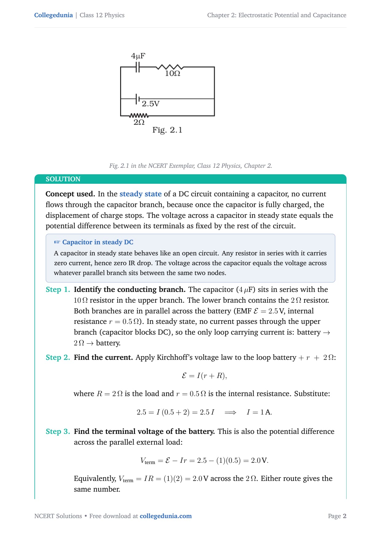
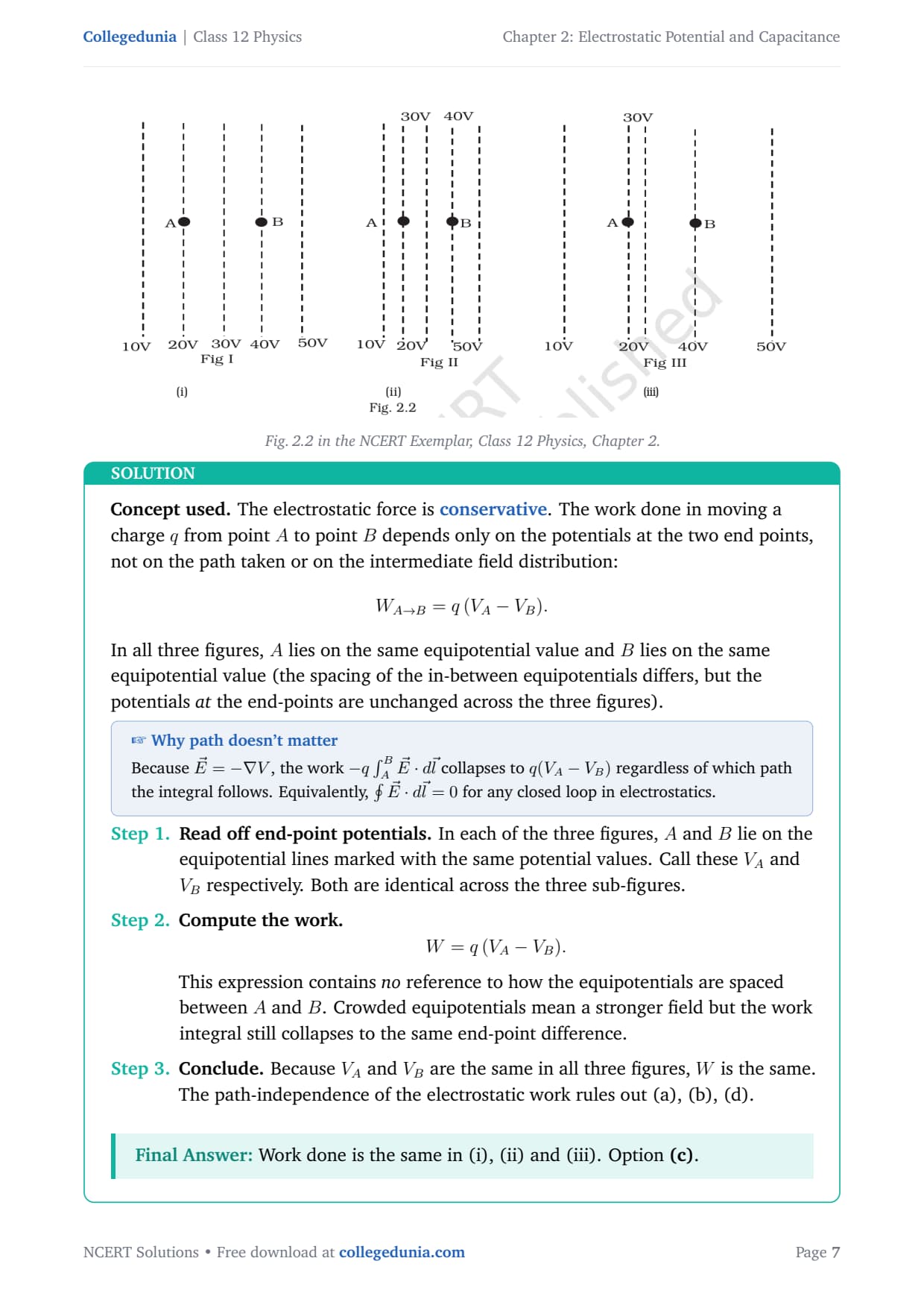
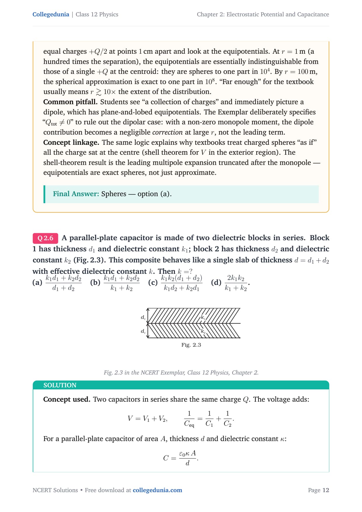
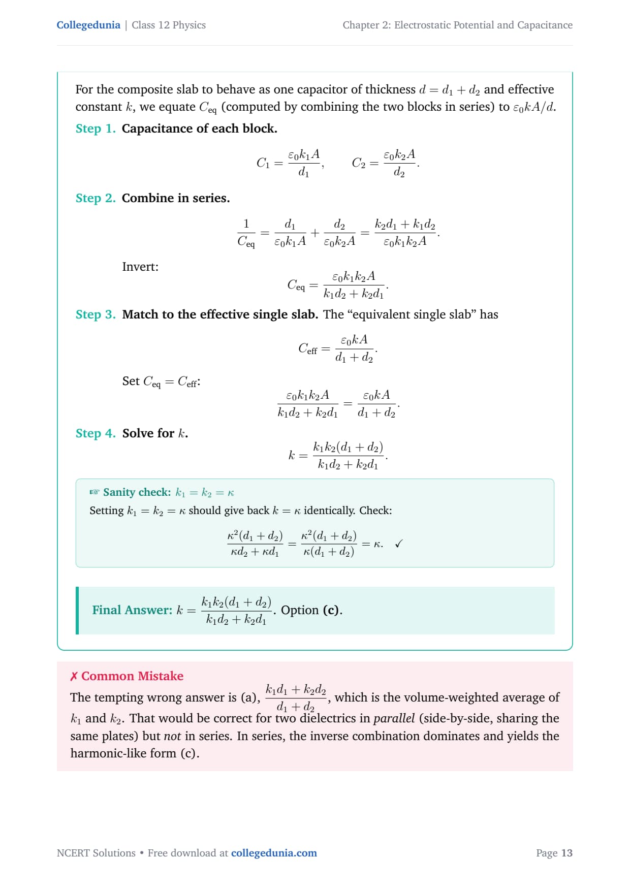
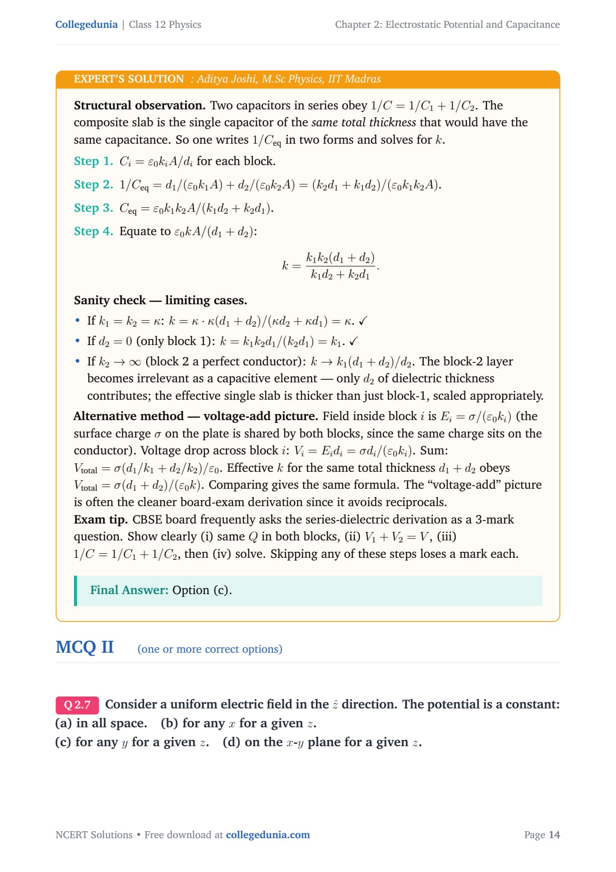
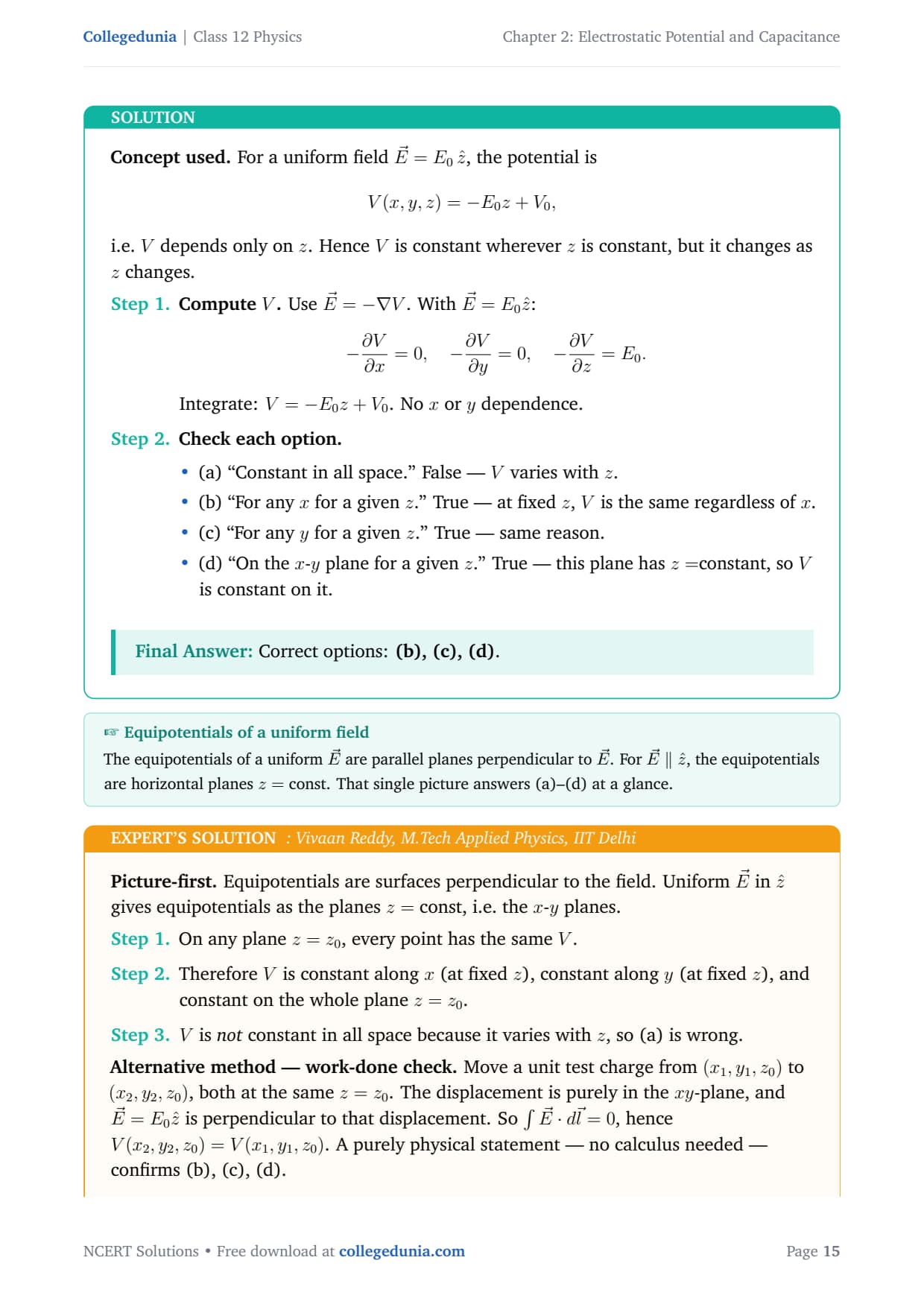
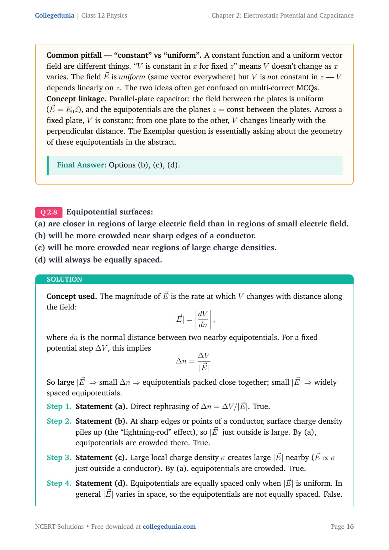

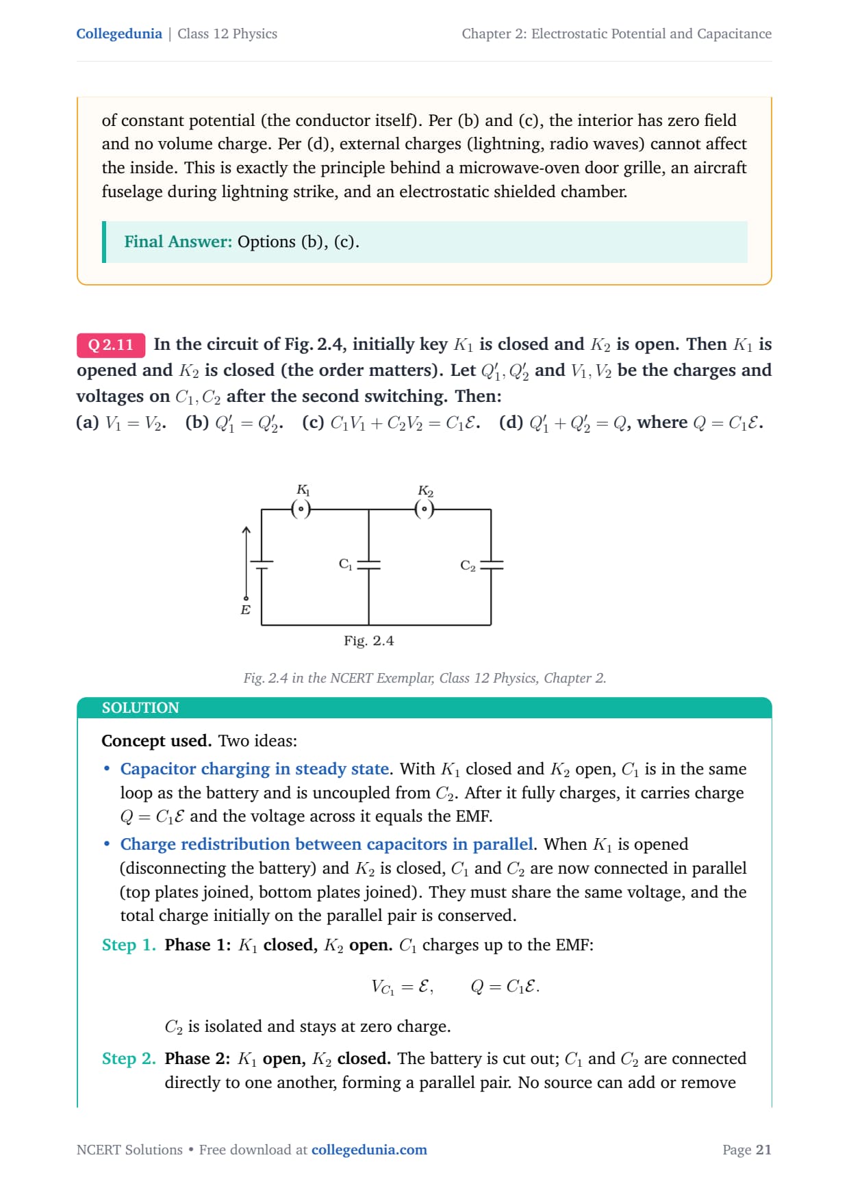
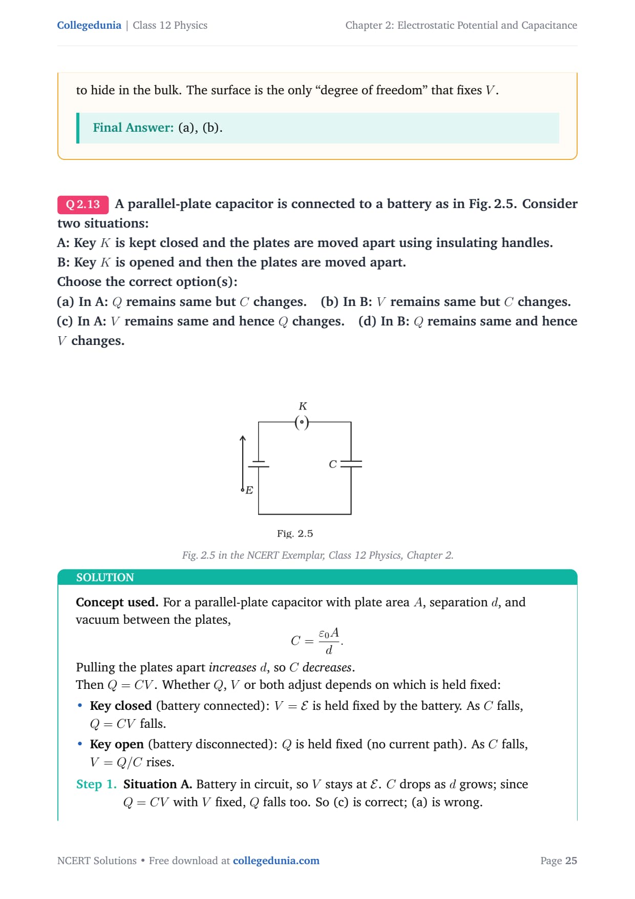
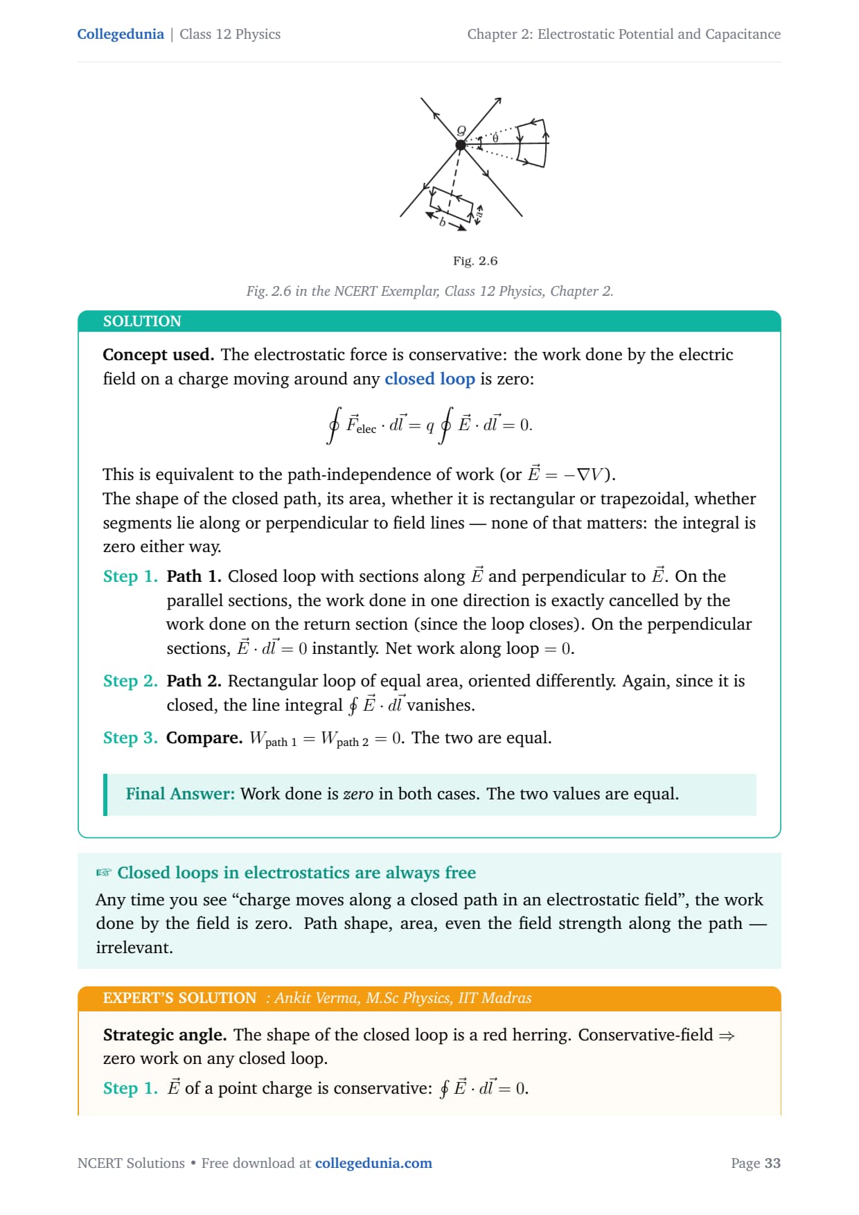
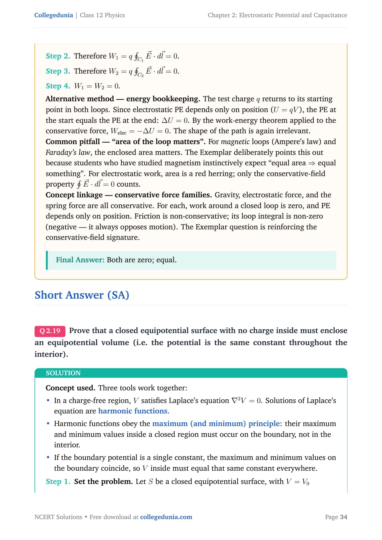
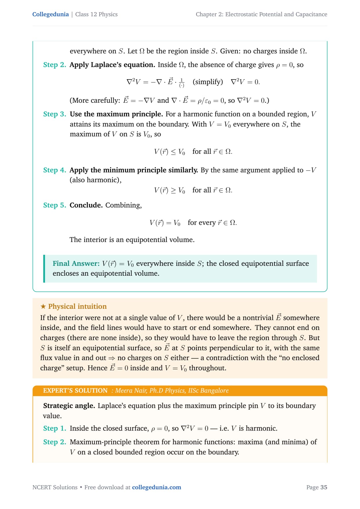
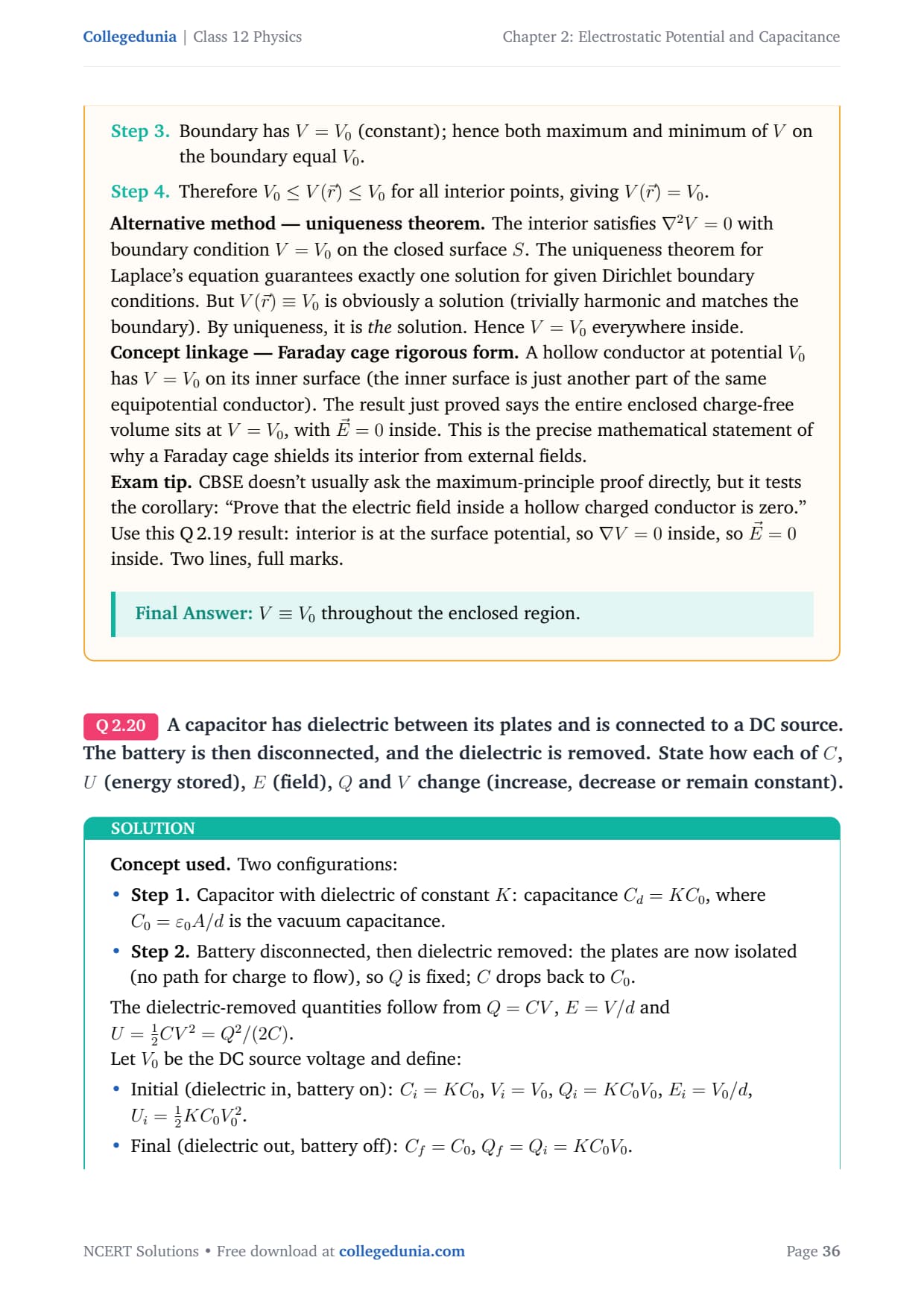
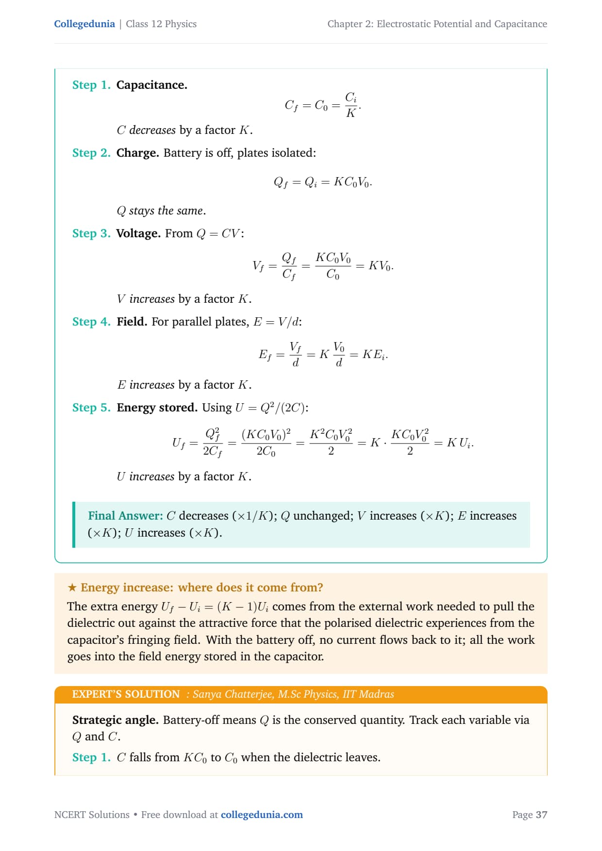
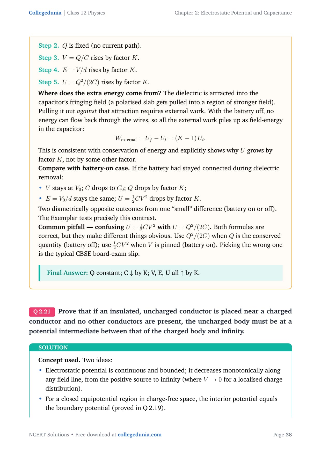
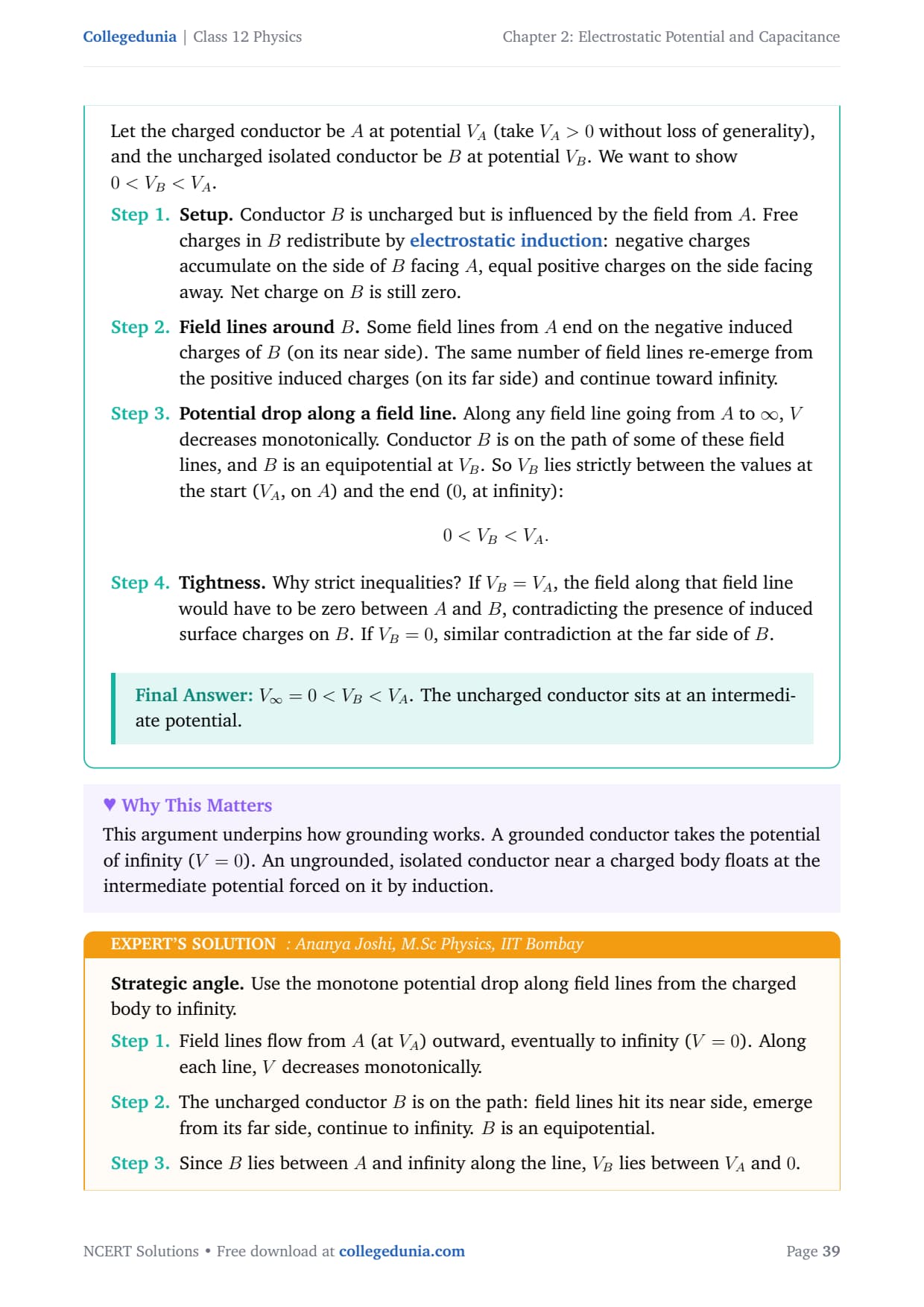
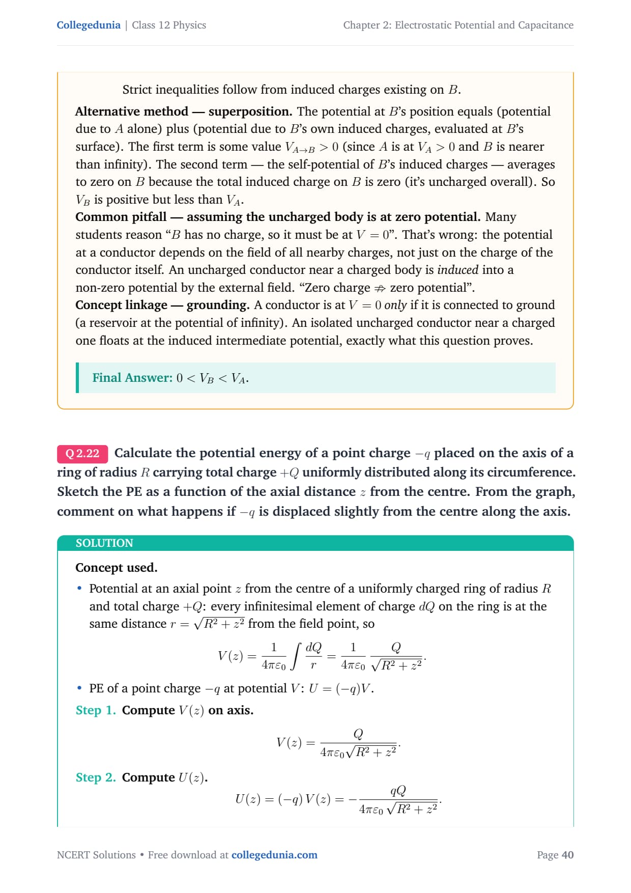
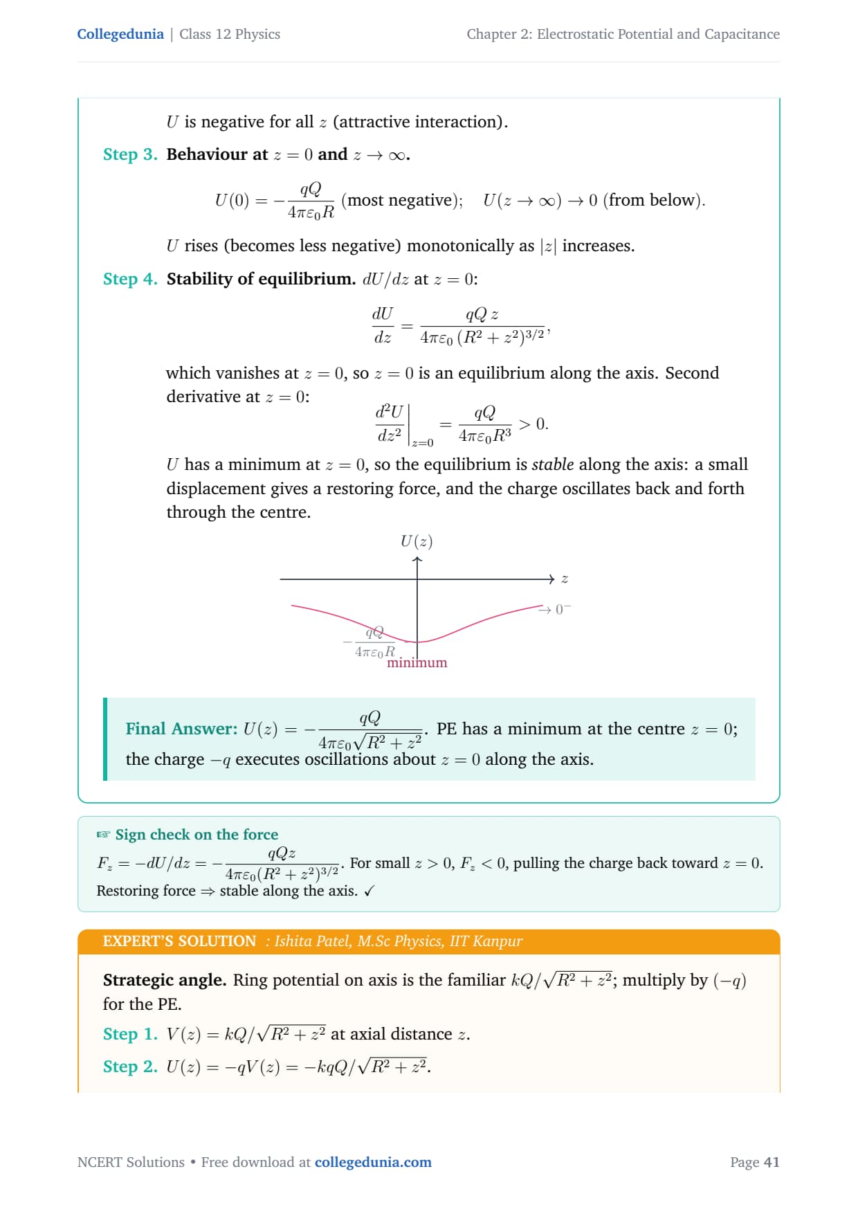
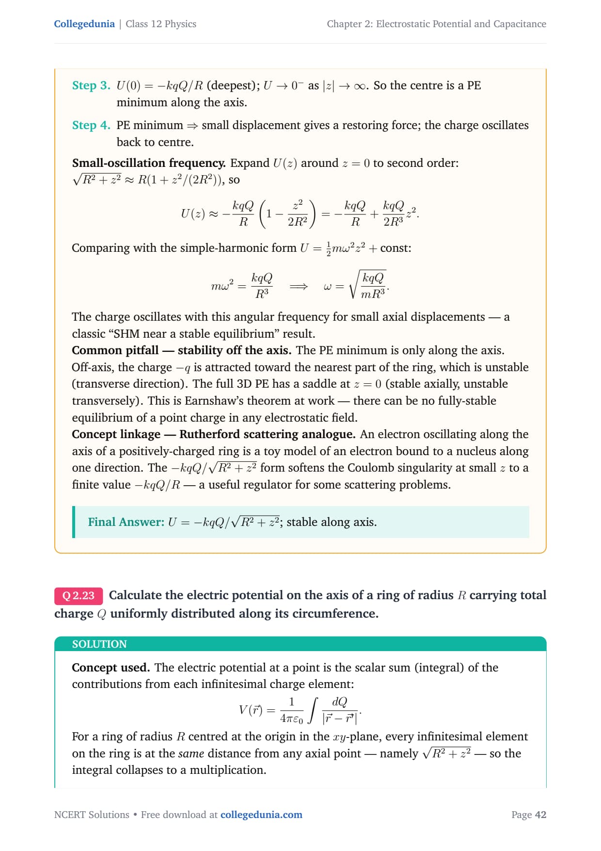
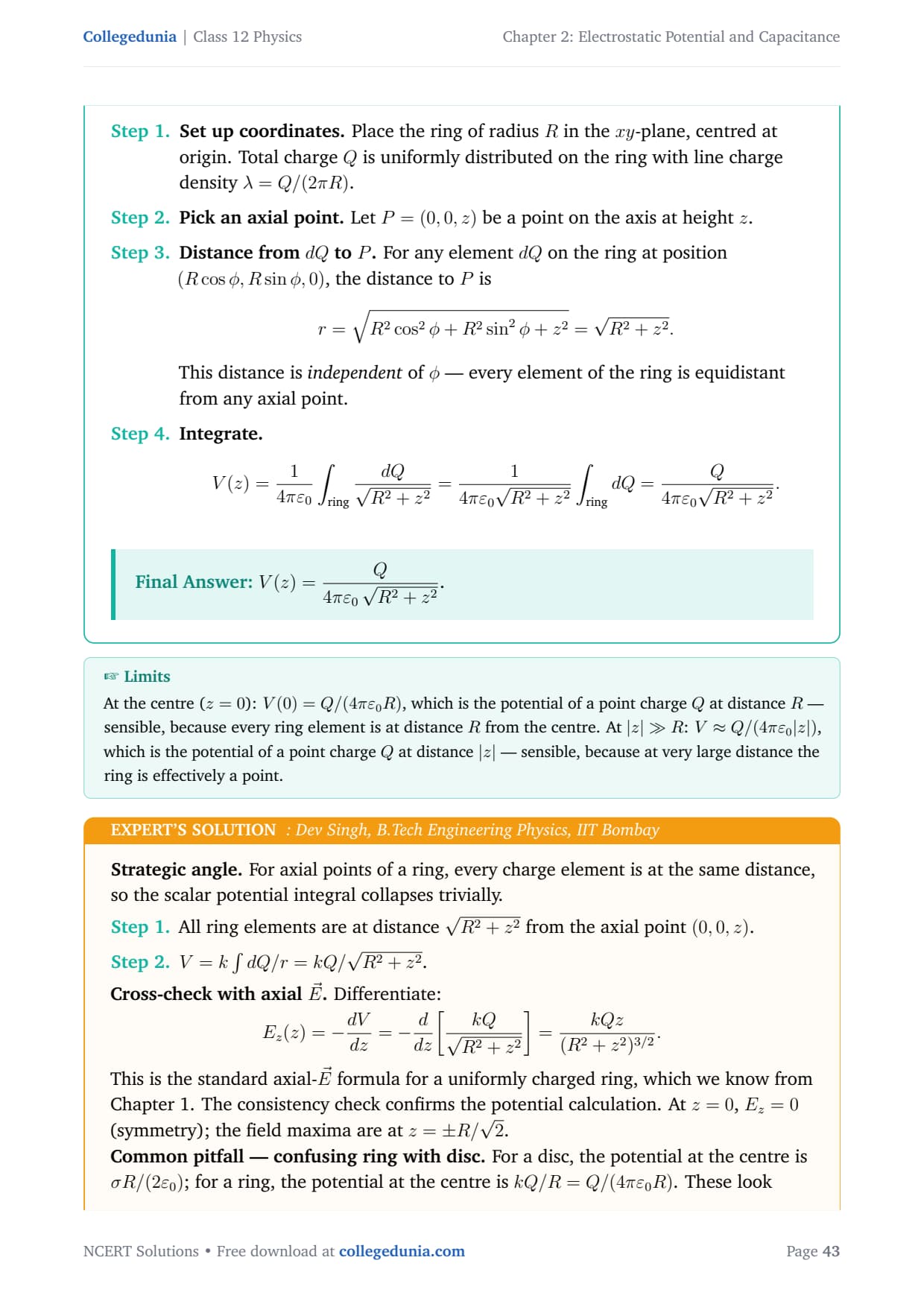
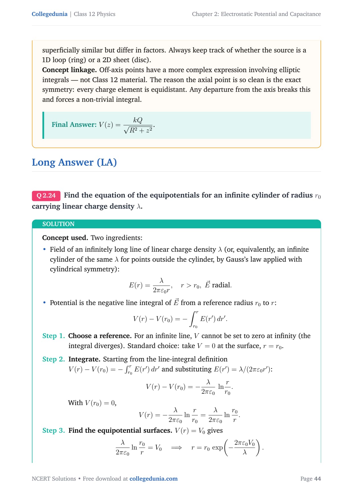
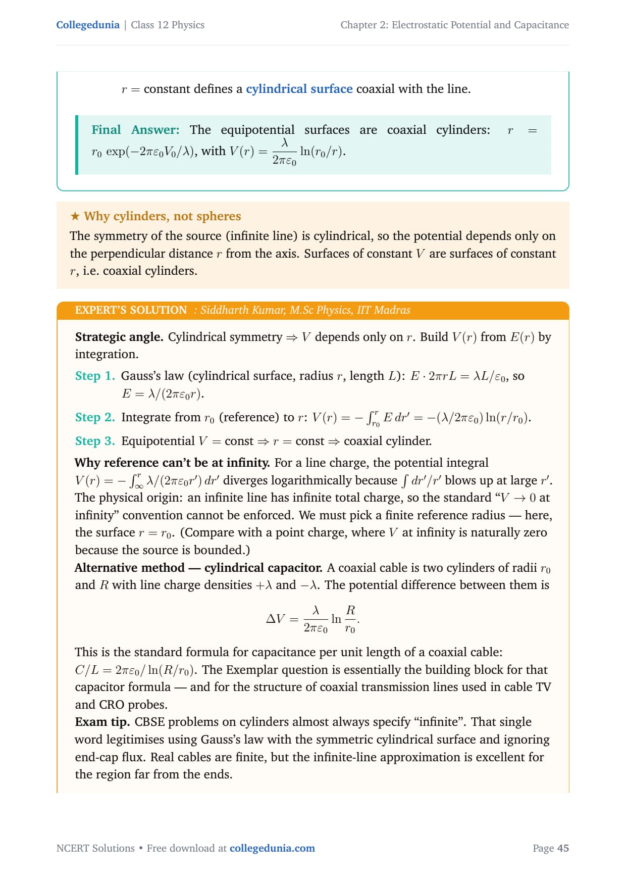
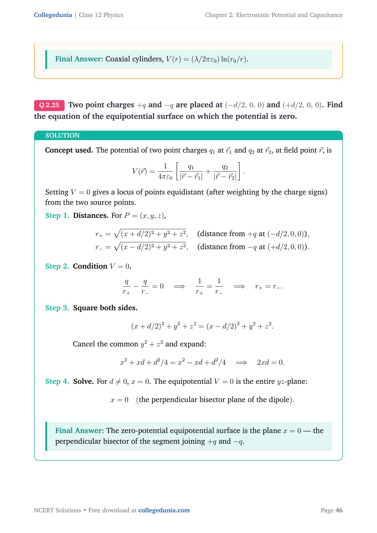
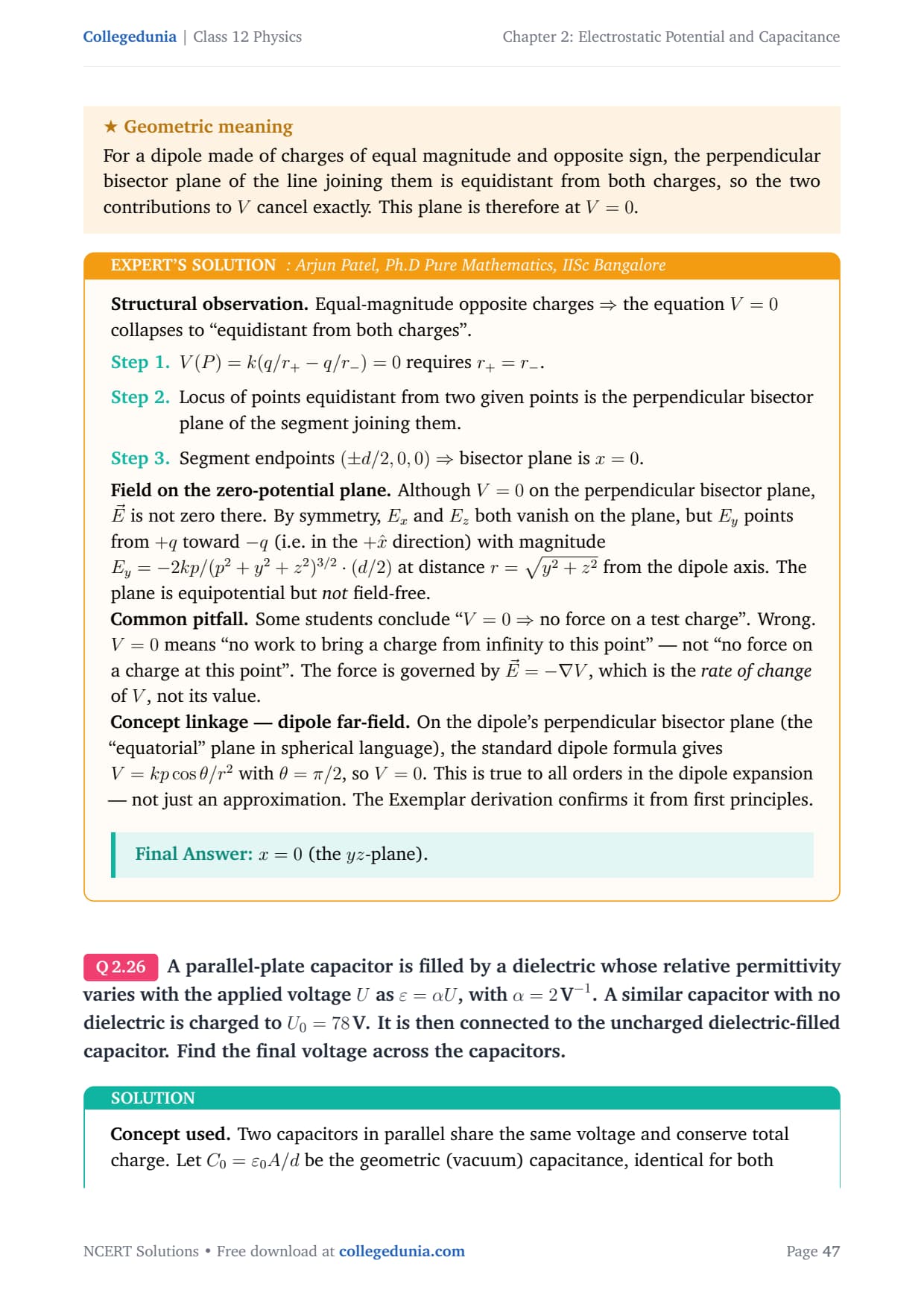
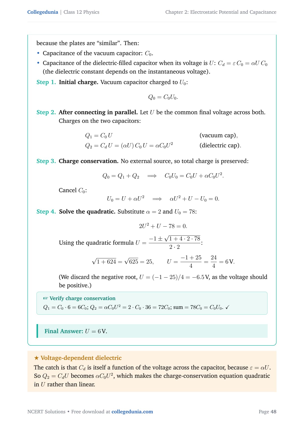
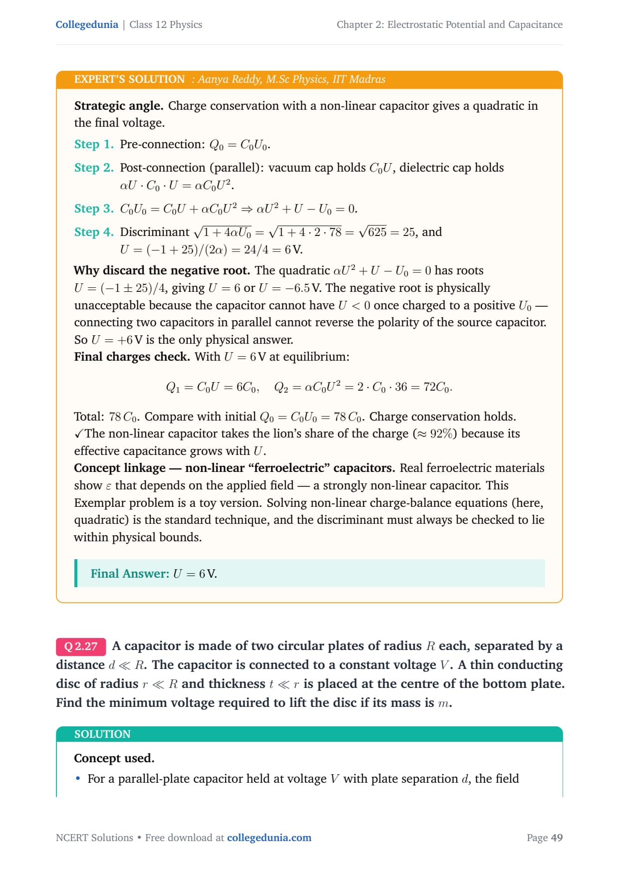
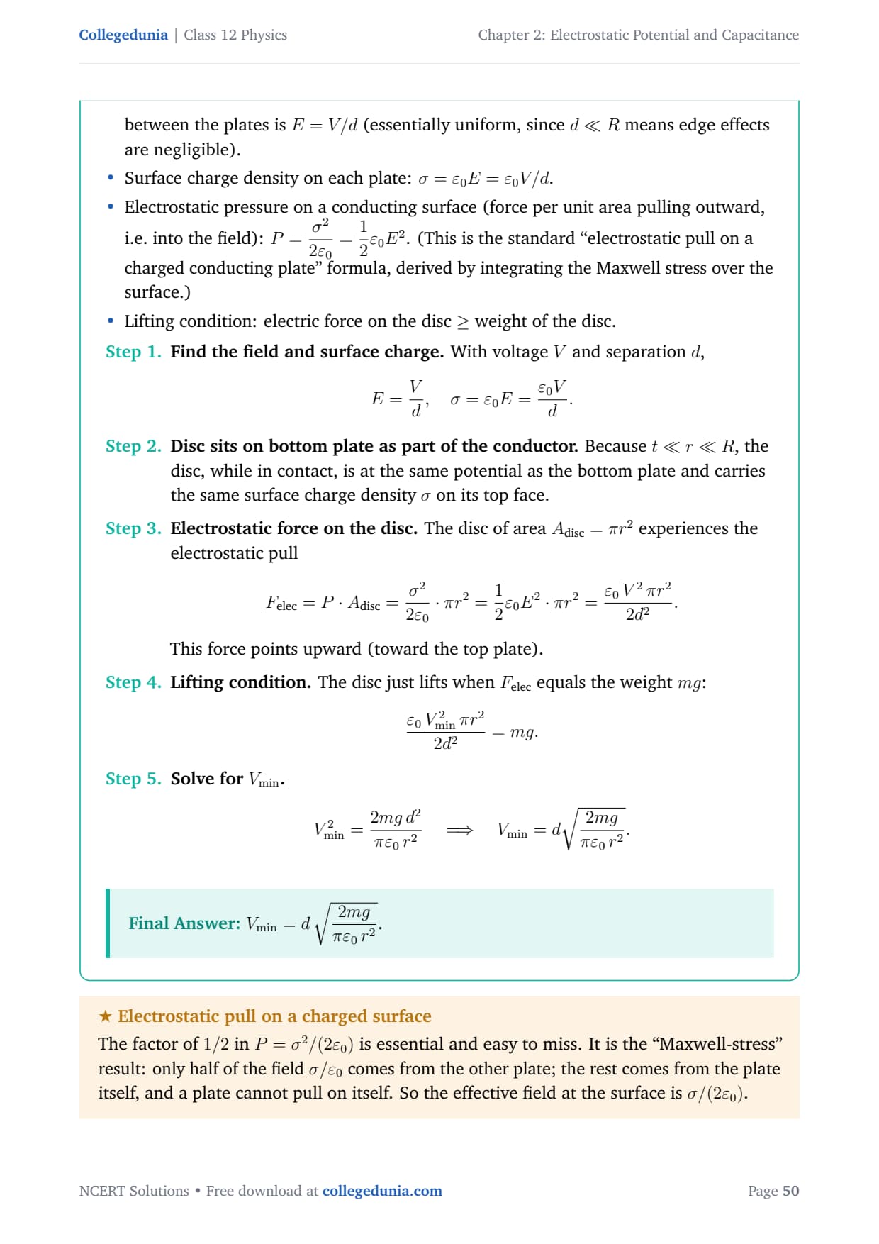
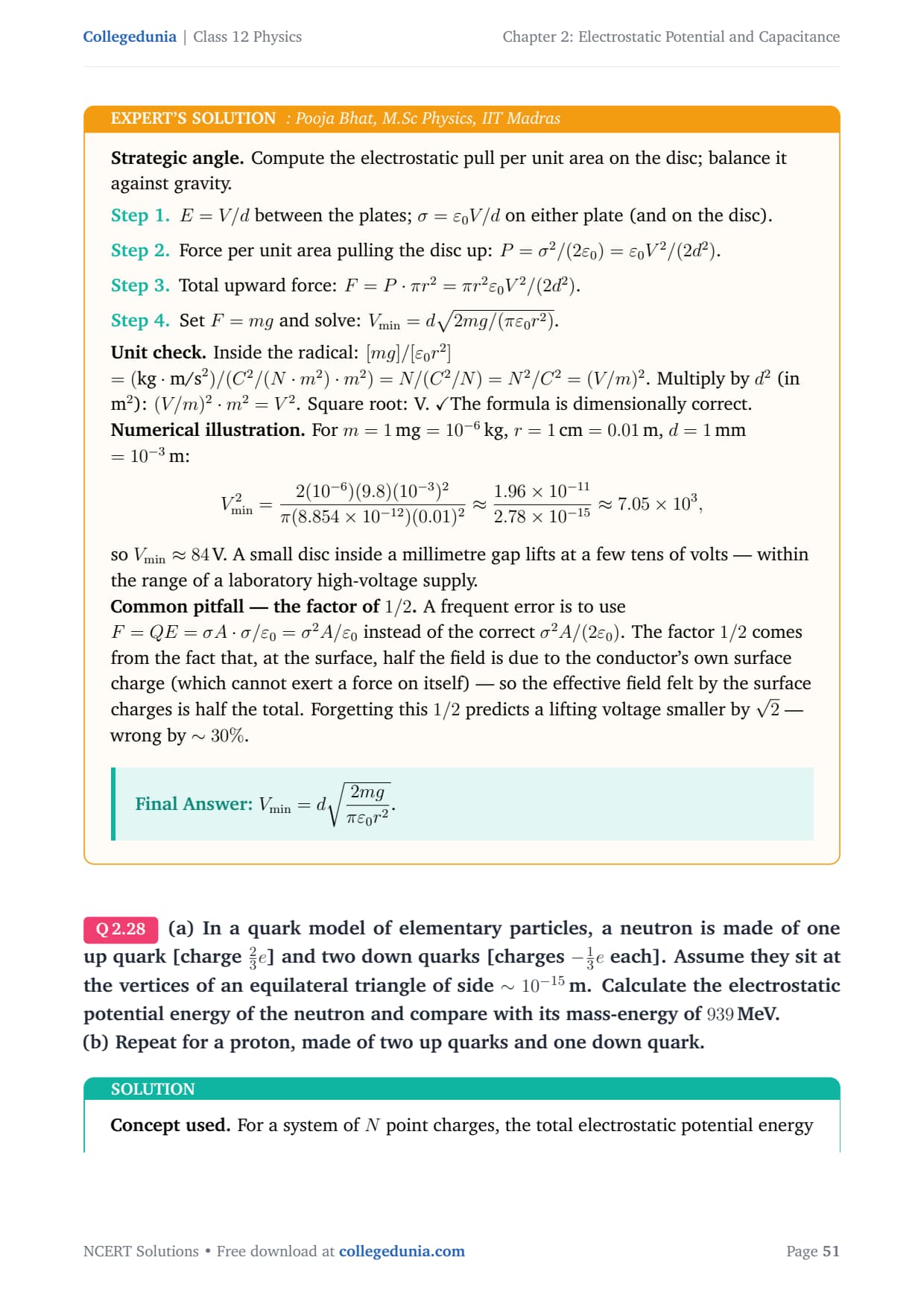
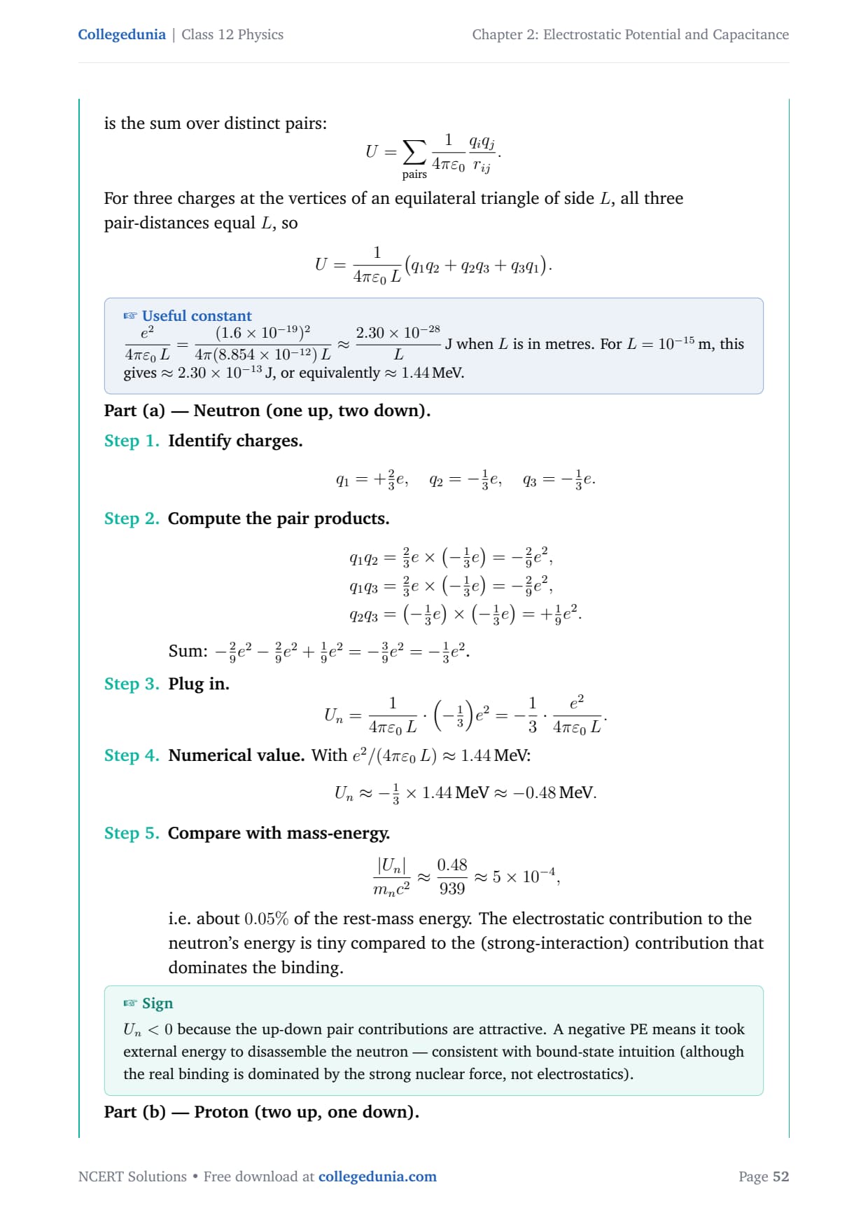
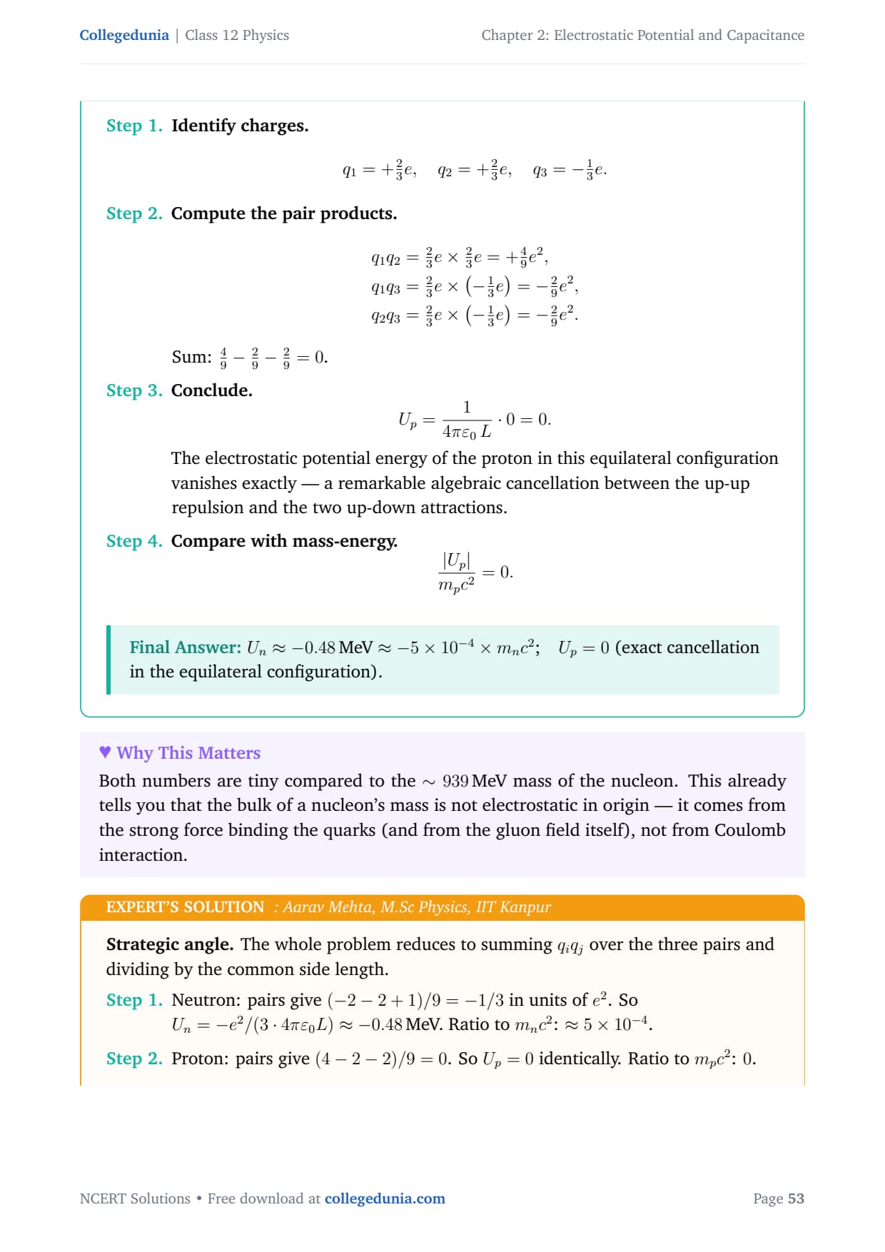
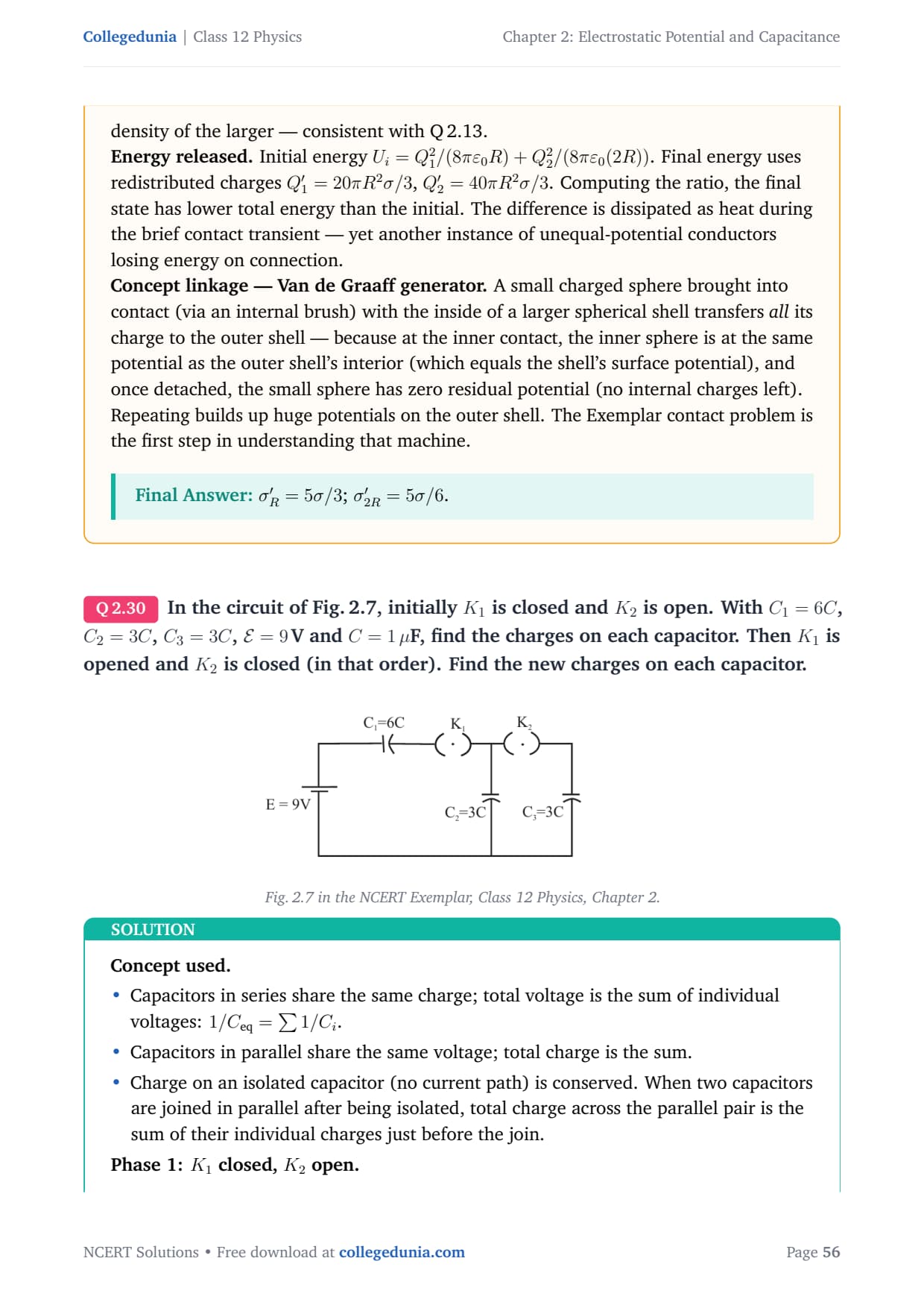
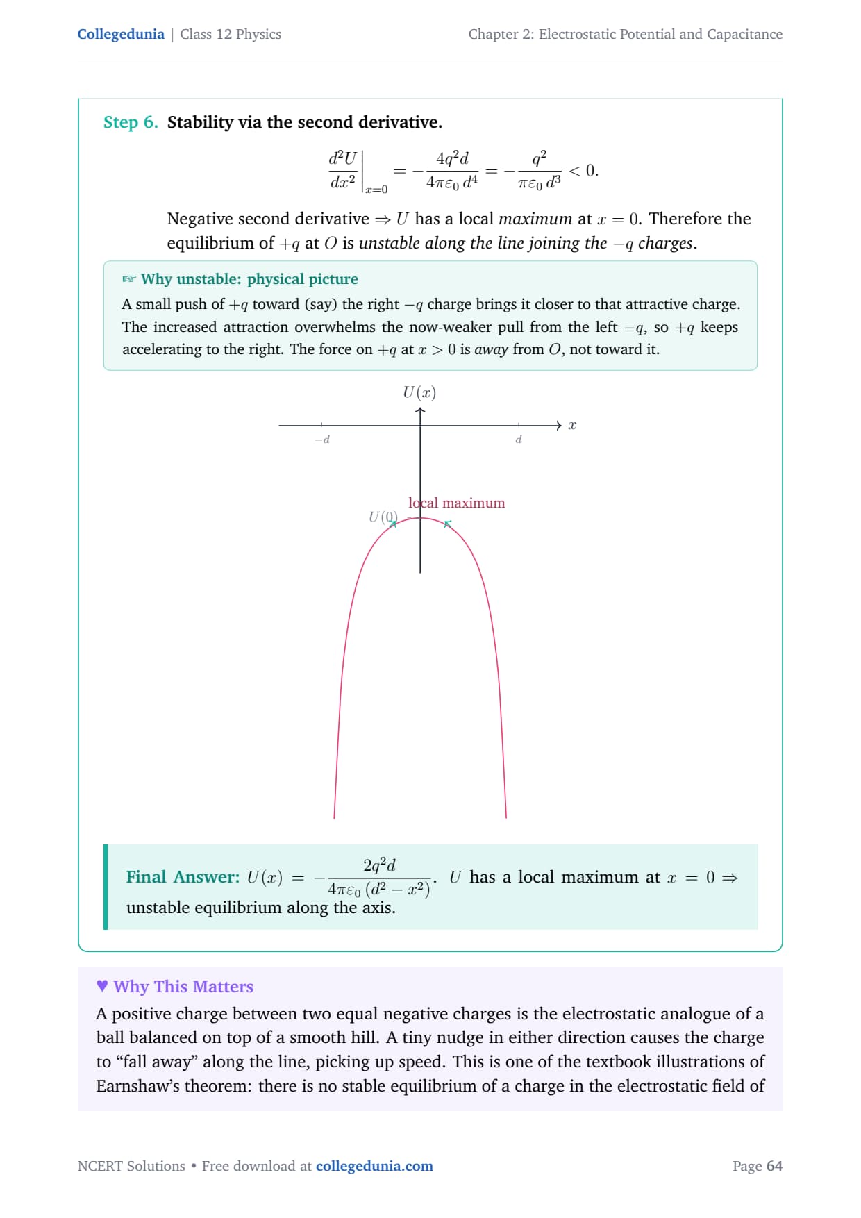





Comments