Junior-Class Mentor, TFI Fellow | Updated 3+ months ago
The NCERT Solutions for Class 10 Maths Chapter 13 Statistics cover every question from Exercise 13.1, 13.2, and 13.3 for the 2026-27 CBSE syllabus. Each grouped-data problem is solved step by step: pick the method, build the table, apply the formula, and reach the mean, median, or mode.
All questions from Exercise 13.1, 13.2, and 13.3 solved, with formula substitution and an Expert Solution that adds exam strategy and common-error warnings.
Full coverage of mean, median, and mode of grouped data: direct, assumed mean, and step-deviation methods, plus cumulative frequency, modal class, and ogive.
What the NCERT Solutions for Class 10 Maths Chapter 13 Statistics Cover
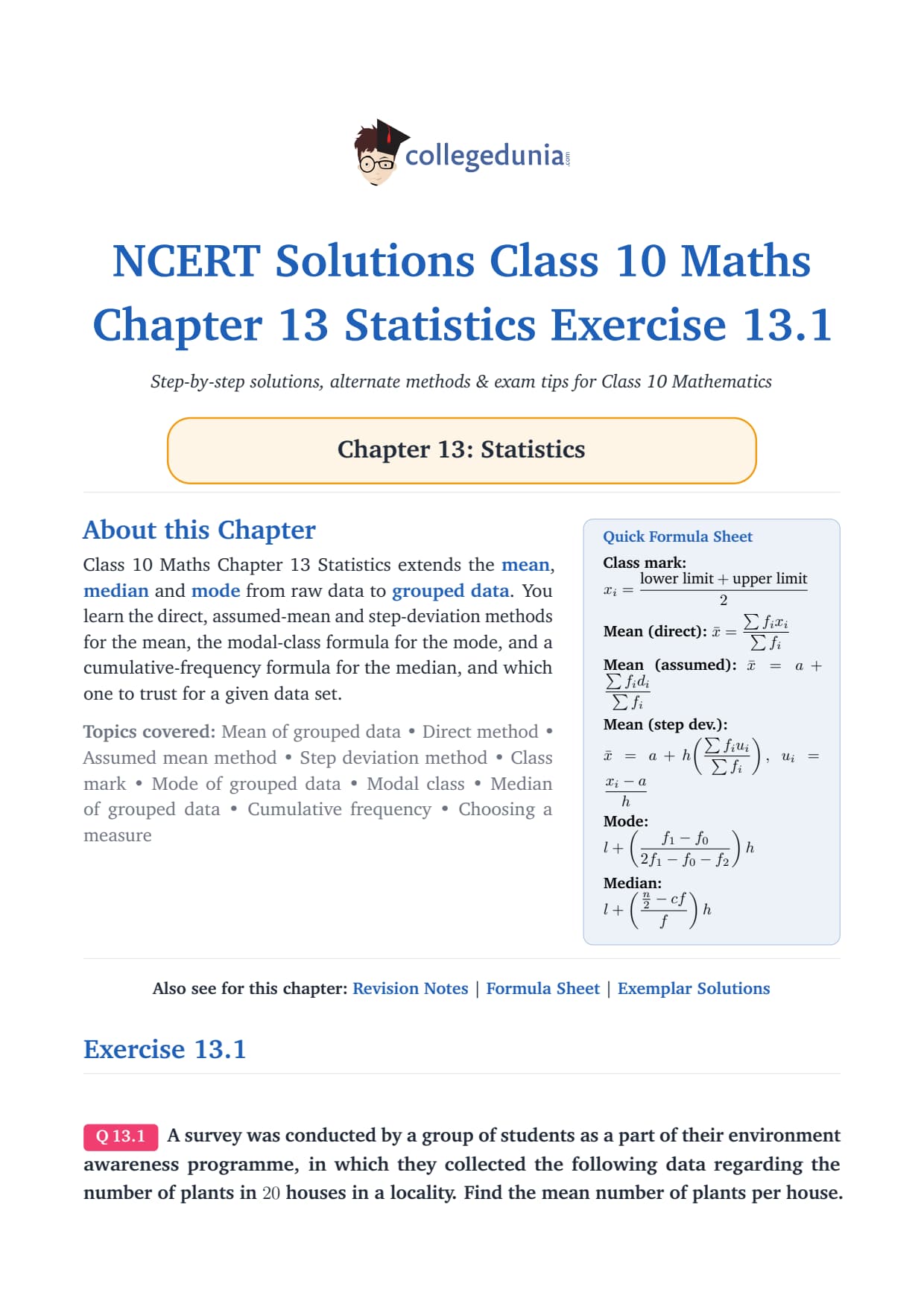
Chapter 13 builds on Class 9 statistics, but now data is grouped into class intervals. So you use the mid-value of each class. The chapter covers three measures of central tendency:
Mean: multiply each mid-value xi by its frequency fi. Three methods give the same answer: direct, assumed mean, and step-deviation.
Mode: the class with the highest frequency is the modal class. The formula uses its frequency and its two neighbours.
Median: build the cumulative frequency (a running total), find the class holding the n/2-th value, then apply the median formula.
Ogive: a cumulative frequency curve that gives the median without the formula.
Key Formulas for Statistics Class 10 Chapter 13 (Mean, Median, Mode)
This table lists every formula you need for the three exercises. Memorise these before the exam. The board gives you the data and expects you to pick and apply the right formula yourself.
Measure
Method
Formula
When to use
Mean
Direct method
x̄ = Σfixi / Σfi
When xi values are small and easy to multiply
Mean
Assumed mean (deviation)
x̄ = a + (Σfidi / Σfi)
When xi values are large; di = xi − a
Mean
Step-deviation
x̄ = a + (Σfiui / Σfi) × h
When class width h is uniform; ui = (xi − a)/h
Mode
Modal class formula
Mode = l + [(f1 − f0) / (2f1 − f0 − f2)] × h
l = lower limit of modal class; f0, f1, f2 = before, modal, after
Median
Median class formula
Median = l + [(n/2 − cf) / f] × h
cf = cumulative frequency before the median class; f = its frequency; h = class width
Quick Tip: For step-deviation, take the assumed mean (a) as the mid-value of the highest-frequency class. This keeps the ui values small and cuts arithmetic errors.
Exercise-Wise Map for Class 10 Maths Chapter 13 Statistics
Each exercise tests one measure. This map shows the questions and the one step that decides your marks.
Exercise
Tests
Questions
Step that decides your marks
13.1
Mean (direct, assumed mean, step-deviation)
9
Find mid-values, build the fixi table, and check Σfi equals n before dividing.
13.2
Mode (modal class)
6
Pick the highest-frequency class as the modal class. Label f0, f1, f2 as before, modal, after.
13.3
Median + ogive
7
Build the cumulative frequency column, find n/2, and use the cf of the class before the median class.
Solved Example: Mean by the Step-Deviation Method
Daily wages of 50 workers fall in classes 500-520 to 580-600 with frequencies 12, 14, 8, 6, 10. Find the mean.
Set up: mid-values 510, 530, 550, 570, 590; class width h = 20; assumed mean a = 550 (the central mid-value).
Related Links: Open the NCERT Solutions for the other chapters of Class 10 Maths below. Each page has the same step-by-step style, PDF download, and FAQ.
All NCERT Solutions for Class 10 Maths Chapter 13 Statistics with Step-by-Step Solutions
Exercise 13.1
Q 13.1
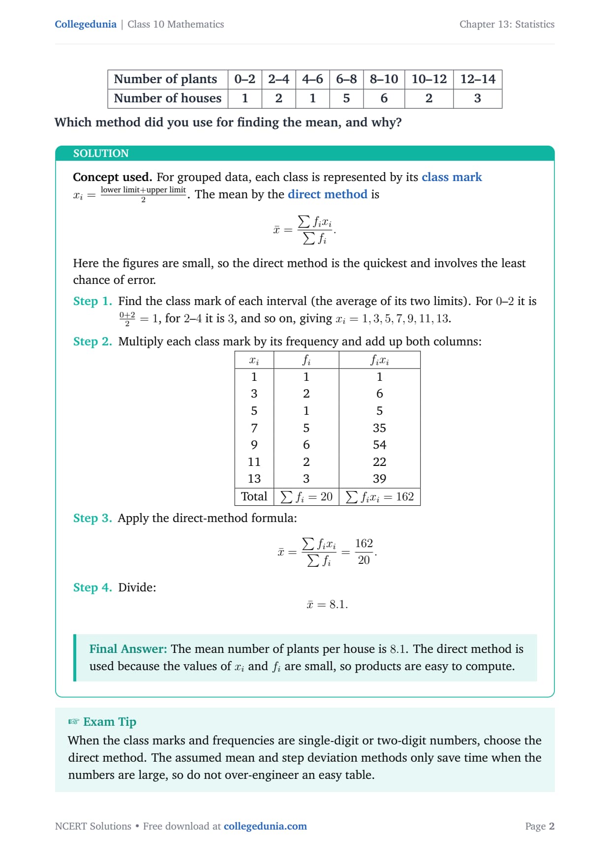
A survey was conducted by a group of students as a part of
their environment awareness programme, in which they collected the
following data regarding the number of plants in 20 houses in a
locality. Find the mean number of plants per house.
tabular|l|c|c|c|c|c|c|c|
Number of plants & 0–2 & 2–4 & 4–6 & 6–8 & 8–10 & 10–12 & 12–14
Number of houses & 1 & 2 & 1 & 5 & 6 & 2 & 3
tabular
Which method did you use for finding the mean, and why?
Concept used. For grouped data, each class is represented by its
class markxi=lower limit+upper limit2.
The mean by the direct method is
x̄=∑ fi xi∑ fi.
Here the figures are small, so the direct method is the quickest and
involves the least chance of error.
Find the class mark of each interval (the average of its two
limits). For 0–2 it is 0+22=1, for 2–4 it
is 3, and so on, giving xi = 1,3,5,7,9,11,13.
Multiply each class mark by its frequency and add up both
columns:
tabular|c|c|c|
xi & fi & fi xi
1 & 1 & 1
3 & 2 & 6
5 & 1 & 5
7 & 5 & 35
9 & 6 & 54
11 & 2 & 22
13 & 3 & 39
Total & ∑ fi=20 & ∑ fi xi=162
tabular
Apply the direct-method formula:
x̄=∑ fi xi∑ fi=16220.
Divide:
x̄=8.1.
The mean number of plants per house is 8.1. The direct method is used because the values of xi and fi are small, so products are easy to compute.
AV
Anjali Verma
M.Sc Mathematics, University of Delhi
Verified Expert
How an examiner reads this answer. Full marks here depend on a
clean three-column table and a stated reason for the method.
Quick check first: the seven classes are equal in width and
the frequencies add to exactly 20 houses, so confirm that total
before any arithmetic begins.
Class-mark idea: taking each class mark as the centre of
its interval treats every house in the 8–10 class as if it had
exactly 9 plants, which is the standard grouped-data assumption.
Why direct: the products fi xi run 1,6,5,35,54,22,39
and total 162; with the largest class mark only 13 and the
largest frequency only 6, these multiplications are trivial, so
the direct method is fastest and least error-prone.
Presentation: write the Total row in bold so the examiner
can verify both column sums at a glance, then quote the single
division that produces the mean.
Sanity check: the answer 8.1 sits between the smallest
class mark 1 and the largest 13, which earns confidence.
x̄=16220=8.1 plants per house, by the direct method.
Q 13.2
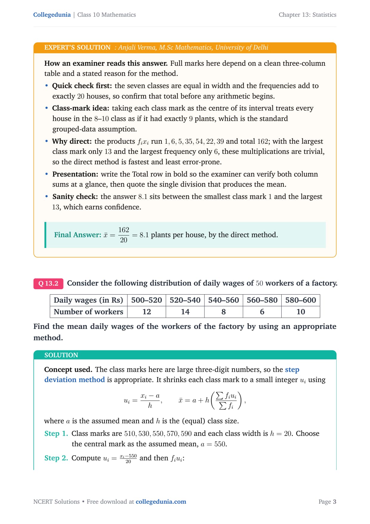
Consider the following distribution of daily wages of 50
workers of a factory.
tabular|l|c|c|c|c|c|
Daily wages (in ) & 500–520 & 520–540 & 540–560 & 560–580 & 580–600
Number of workers & 12 & 14 & 8 & 6 & 10
tabular
Find the mean daily wages of the workers of the factory by using an
appropriate method.
Concept used. The class marks here are large three-digit
numbers, so the step deviation method is appropriate. It
shrinks each class mark to a small integer ui using
ui=xi-ah, x̄=a+h(∑ fi ui∑ fi),
where a is the assumed mean and h is the (equal) class size.
Class marks are 510,530,550,570,590 and each class width is
h=20. Choose the central mark as the assumed mean, a=550.
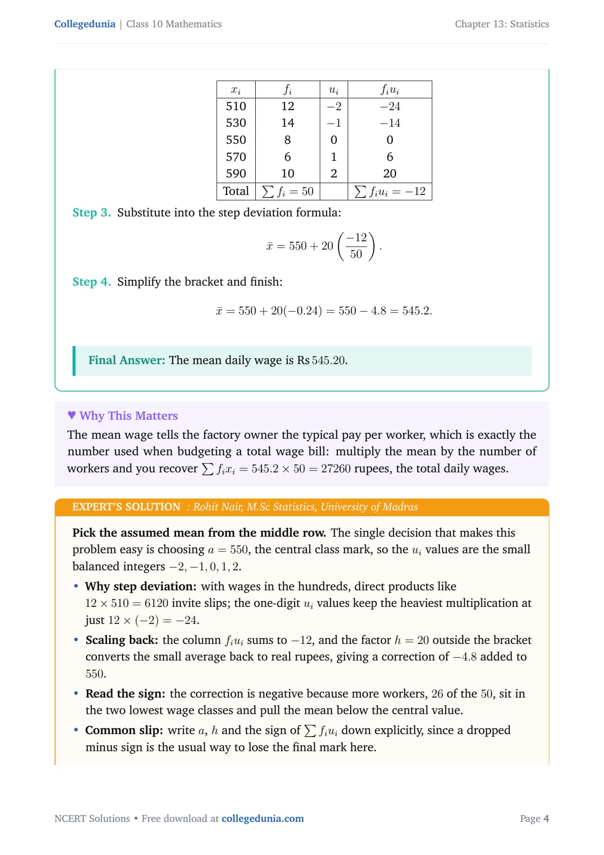
Substitute into the step deviation formula:
x̄=550+20(-1250).
Simplify the bracket and finish:
x̄=550+20(-0.24)=550-4.8=545.2.
The mean daily wage is 545.20.
RN
Rohit Nair
M.Sc Statistics, University of Madras
Verified Expert
Pick the assumed mean from the middle row. The single decision
that makes this problem easy is choosing a=550, the central class mark, so
the ui values are the small balanced integers -2,-1,0,1,2.
Why step deviation: with wages in the hundreds, direct
products like 12× 510 = 6120 invite slips; the one-digit
ui values keep the heaviest multiplication at just
12×(-2)=-24.
Scaling back: the column fi ui sums to -12, and the
factor h=20 outside the bracket converts the small average back to
real rupees, giving a correction of -4.8 added to 550.
Read the sign: the correction is negative because more
workers, 26 of the 50, sit in the two lowest wage classes and
pull the mean below the central value.
Common slip: write a, h and the sign of ∑ fi ui
down explicitly, since a dropped minus sign is the usual way to lose
the final mark here.
x̄=550+20(-1250)=545.2 rupees.
Q 13.3
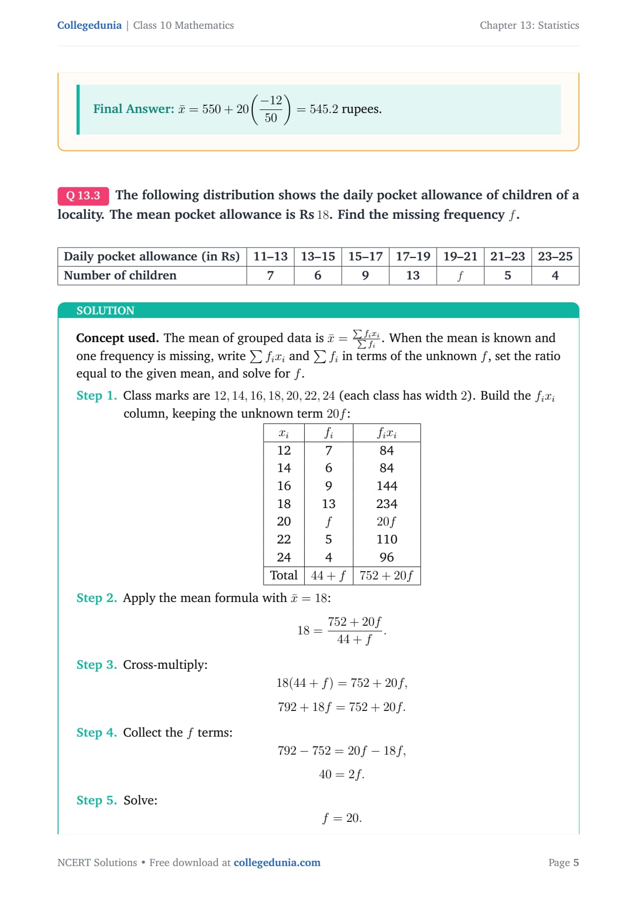
The following distribution shows the daily pocket allowance of
children of a locality. The mean pocket allowance is 18. Find
the missing frequency f.
!%
tabular|l|c|c|c|c|c|c|c|
Daily pocket allowance (in ) & 11–13 & 13–15 & 15–17 & 17–19 & 19–21 & 21–23 & 23–25
Number of children & 7 & 6 & 9 & 13 & f & 5 & 4
tabular
Concept used. The mean of grouped data is
x̄=∑ fi xi∑ fi. When the mean is known and one
frequency is missing, write ∑ fi xi and ∑ fi in terms of the
unknown f, set the ratio equal to the given mean, and solve for f.
Class marks are 12,14,16,18,20,22,24 (each class has width 2).
Build the fi xi column, keeping the unknown term 20f:
tabular|c|c|c|
xi & fi & fi xi
12 & 7 & 84
14 & 6 & 84
16 & 9 & 144
18 & 13 & 234
20 & f & 20f
22 & 5 & 110
24 & 4 & 96
Total & 44+f & 752+20f
tabular
Apply the mean formula with x̄=18:
18=752+20f44+f.
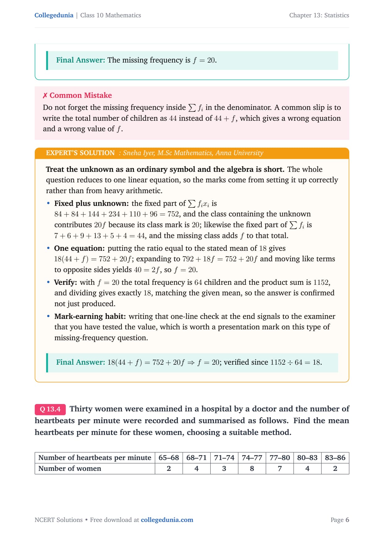
Treat the unknown as an ordinary symbol and the algebra is short.
The whole question reduces to one linear equation, so the marks come from
setting it up correctly rather than from heavy arithmetic.
Fixed plus unknown: the fixed part of ∑ fi xi is
84+84+144+234+110+96=752, and the class containing the unknown
contributes 20f because its class mark is 20; likewise the fixed
part of ∑ fi is 7+6+9+13+5+4=44, and the missing class adds
f to that total.
One equation: putting the ratio equal to the stated mean of
18 gives 18(44+f)=752+20f; expanding to 792+18f=752+20f and
moving like terms to opposite sides yields 40=2f, so f=20.
Verify: with f=20 the total frequency is 64 children
and the product sum is 1152, and dividing gives exactly 18,
matching the given mean, so the answer is confirmed not just
produced.
Mark-earning habit: writing that one-line check at the end
signals to the examiner that you have tested the value, which is
worth a presentation mark on this type of missing-frequency
question.
18(44+f)=752+20f⇒ f=20; verified since 1152÷ 64=18.
Q 13.4
Thirty women were examined in a hospital by a doctor and the
number of heartbeats per minute were recorded and summarised as follows.
Find the mean heartbeats per minute for these women, choosing a suitable
method.
!%
tabular|l|c|c|c|c|c|c|c|
Number of heartbeats per minute & 65–68 & 68–71 & 71–74 & 74–77 & 77–80 & 80–83 & 83–86
Number of women & 2 & 4 & 3 & 8 & 7 & 4 & 2
tabular
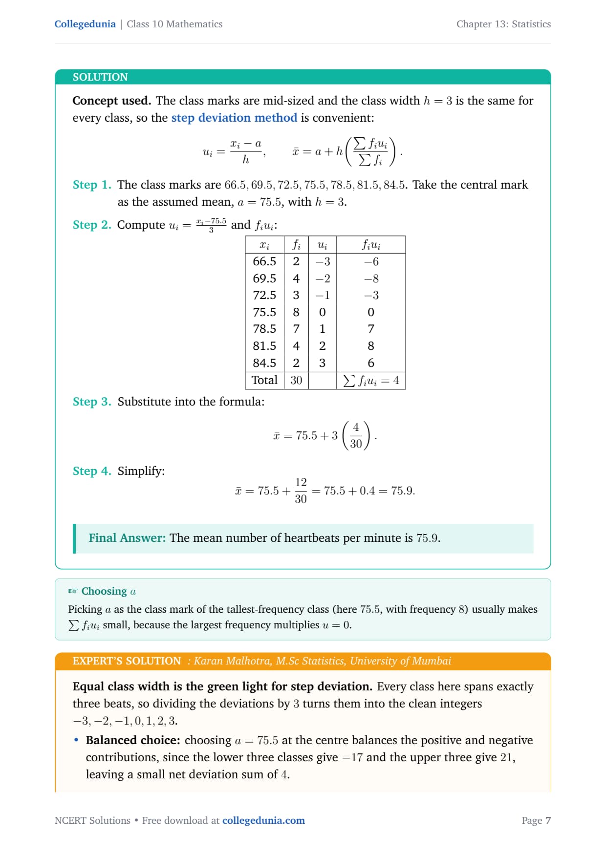
Concept used. The class marks are mid-sized and the class width
h=3 is the same for every class, so the step deviation
method is convenient:
ui=xi-ah, x̄=a+h(∑ fi ui∑ fi).
The class marks are 66.5,69.5,72.5,75.5,78.5,81.5,84.5. Take the
central mark as the assumed mean, a=75.5, with h=3.
Equal class width is the green light for step deviation. Every
class here spans exactly three beats, so dividing the deviations by 3 turns
them into the clean integers -3,-2,-1,0,1,2,3.
Balanced choice: choosing a=75.5 at the centre balances
the positive and negative contributions, since the lower three
classes give -17 and the upper three give 21, leaving a small
net deviation sum of 4.
Scaling: multiplying by the width h=3 and dividing by the
30 women scales this back to a correction of 0.4 beats just above
the assumed mean, so the mean works out to 75.9.
Why it is sensible: the result being close to 75.5 is
exactly what we expect, because the frequencies are nearly symmetric
about the middle class.
Presentation: quote the assumed mean and class size on
their own line before the table, because a mislabelled ui column
is the usual reason this style of answer loses a mark.
x̄=75.5+3(430)=75.9 beats per minute.
Q 13.5
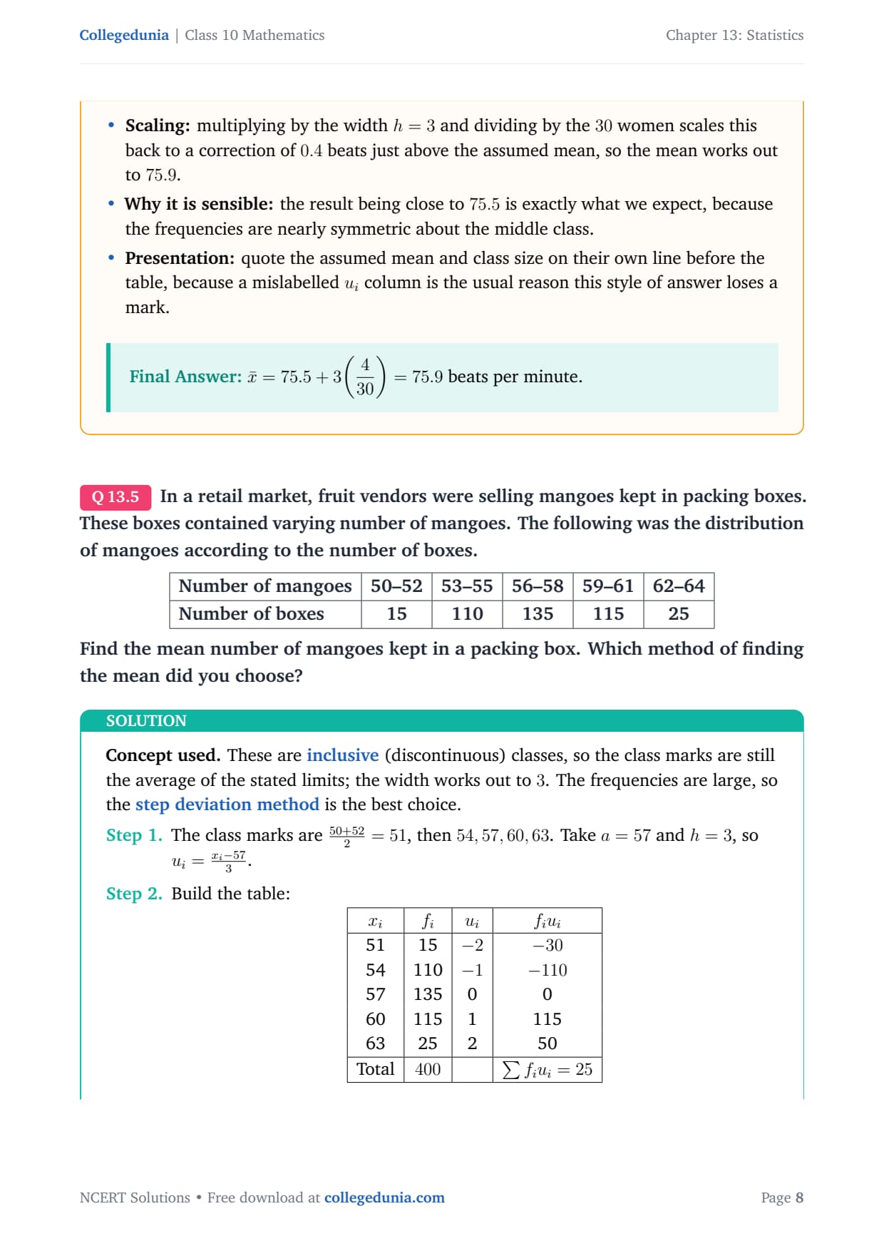
In a retail market, fruit vendors were selling mangoes kept in
packing boxes. These boxes contained varying number of mangoes. The
following was the distribution of mangoes according to the number of
boxes.
tabular|l|c|c|c|c|c|
Number of mangoes & 50–52 & 53–55 & 56–58 & 59–61 & 62–64
Number of boxes & 15 & 110 & 135 & 115 & 25
tabular
Find the mean number of mangoes kept in a packing box. Which method of
finding the mean did you choose?
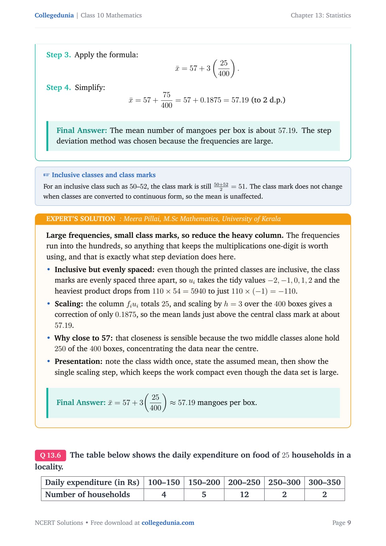
Concept used. These are inclusive (discontinuous)
classes, so the class marks are still the average of the stated limits;
the width works out to 3. The frequencies are large, so the
step deviation method is the best choice.
The class marks are 50+522=51, then 54,57,60,63.
Take a=57 and h=3, so ui=xi-573.
The mean number of mangoes per box is about 57.19. The step deviation method was chosen because the frequencies are large.
MP
Meera Pillai
M.Sc Mathematics, University of Kerala
Verified Expert
Large frequencies, small class marks, so reduce the heavy column.
The frequencies run into the hundreds, so anything that keeps the
multiplications one-digit is worth using, and that is exactly what step
deviation does here.
Inclusive but evenly spaced: even though the printed
classes are inclusive, the class marks are evenly spaced three apart,
so ui takes the tidy values -2,-1,0,1,2 and the heaviest product
drops from 110× 54 = 5940 to just 110×(-1)=-110.
Scaling: the column fi ui totals 25, and scaling by
h=3 over the 400 boxes gives a correction of only 0.1875, so
the mean lands just above the central class mark at about 57.19.
Why close to 57: that closeness is sensible because the two
middle classes alone hold 250 of the 400 boxes, concentrating the
data near the centre.
Presentation: note the class width once, state the assumed
mean, then show the single scaling step, which keeps the work compact
even though the data set is large.
x̄=57+3(25400)≈ 57.19 mangoes per box.
Q 13.6
The table below shows the daily expenditure on food of 25
households in a locality.
tabular|l|c|c|c|c|c|
Daily expenditure (in ) & 100–150 & 150–200 & 200–250 & 250–300 & 300–350
Number of households & 4 & 5 & 12 & 2 & 2
tabular
Find the mean daily expenditure on food by a suitable method.
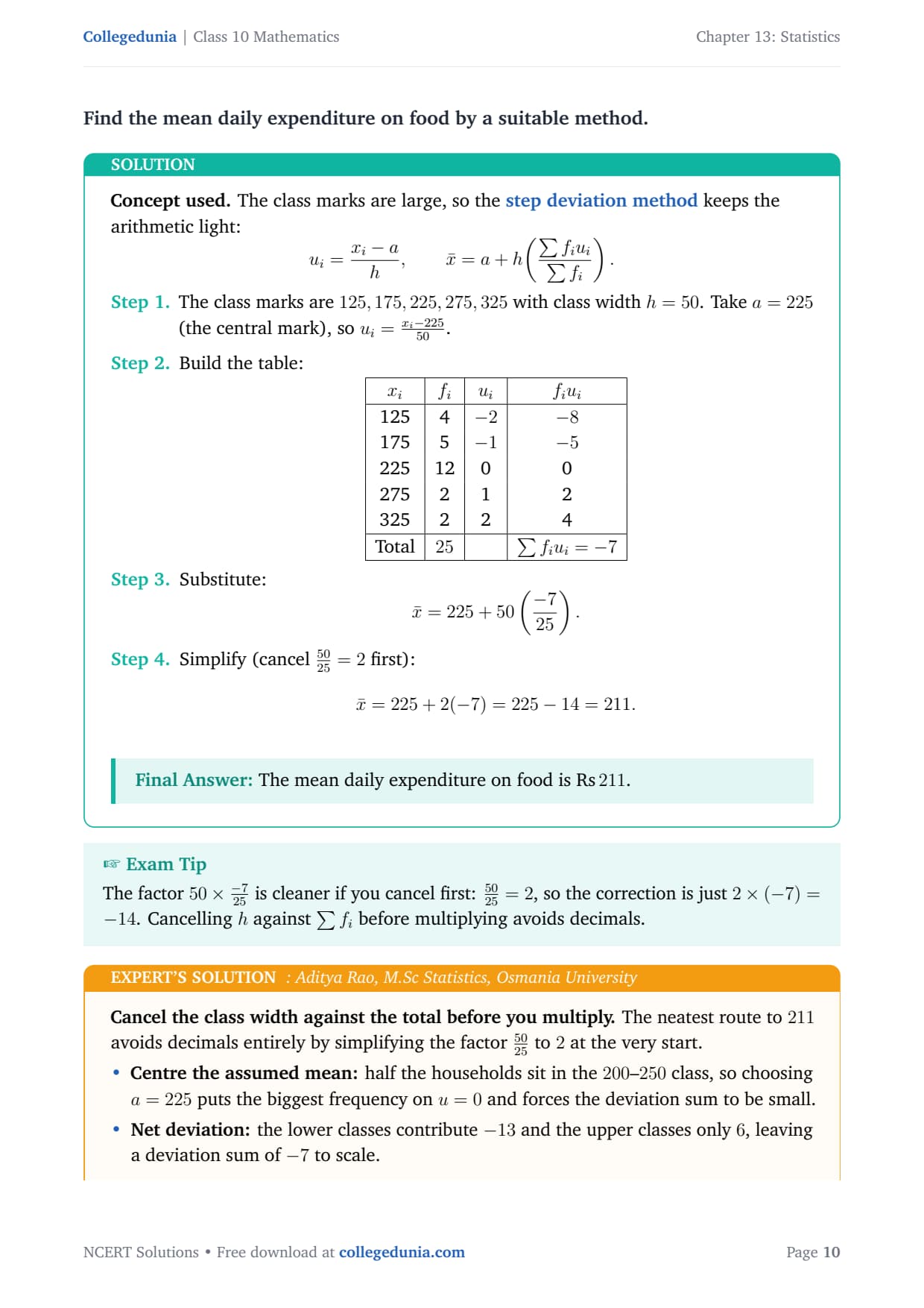
Concept used. The class marks are large, so the step
deviation method keeps the arithmetic light:
ui=xi-ah, x̄=a+h(∑ fi ui∑ fi).
The class marks are 125,175,225,275,325 with class width
h=50. Take a=225 (the central mark), so ui=xi-22550.
Cancel the class width against the total before you multiply. The
neatest route to 211 avoids decimals entirely by simplifying the factor
5025 to 2 at the very start.
Centre the assumed mean: half the households sit in the
200–250 class, so choosing a=225 puts the biggest frequency on
u=0 and forces the deviation sum to be small.
Net deviation: the lower classes contribute -13 and the
upper classes only 6, leaving a deviation sum of -7 to scale.
Cancel then multiply: the correction becomes simply
2×(-7)=-14, so the mean drops to 211, below the central
mark, which matches the data being skewed toward lower expenditure.
Name the method: the question asks for a suitable method, so
state step deviation and the reason of large class marks, because
naming it shows the examiner the choice was deliberate and earns a
presentation mark.
x̄=225+2(-7)= 211 per household per day.
Q 13.7
To find out the concentration of in the air (in parts
per million, i.e., ppm), the data was collected for 30 localities in a
certain city and is presented below:
tabular|l|c|
Concentration of (in ppm) & Frequency
0.00–0.04 & 4
0.04–0.08 & 9
0.08–0.12 & 9
0.12–0.16 & 2
0.16–0.20 & 4
0.20–0.24 & 2
tabular
Find the mean concentration of in the air.
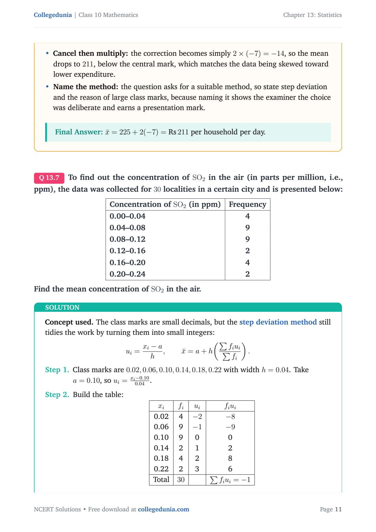
Concept used. The class marks are small decimals, but the
step deviation method still tidies the work by turning them into
small integers:
ui=xi-ah, x̄=a+h(∑ fi ui∑ fi).
Class marks are 0.02,0.06,0.10,0.14,0.18,0.22 with width
h=0.04. Take a=0.10, so ui=xi-0.100.04.
M.Sc Mathematics, Savitribai Phule Pune University
Verified Expert
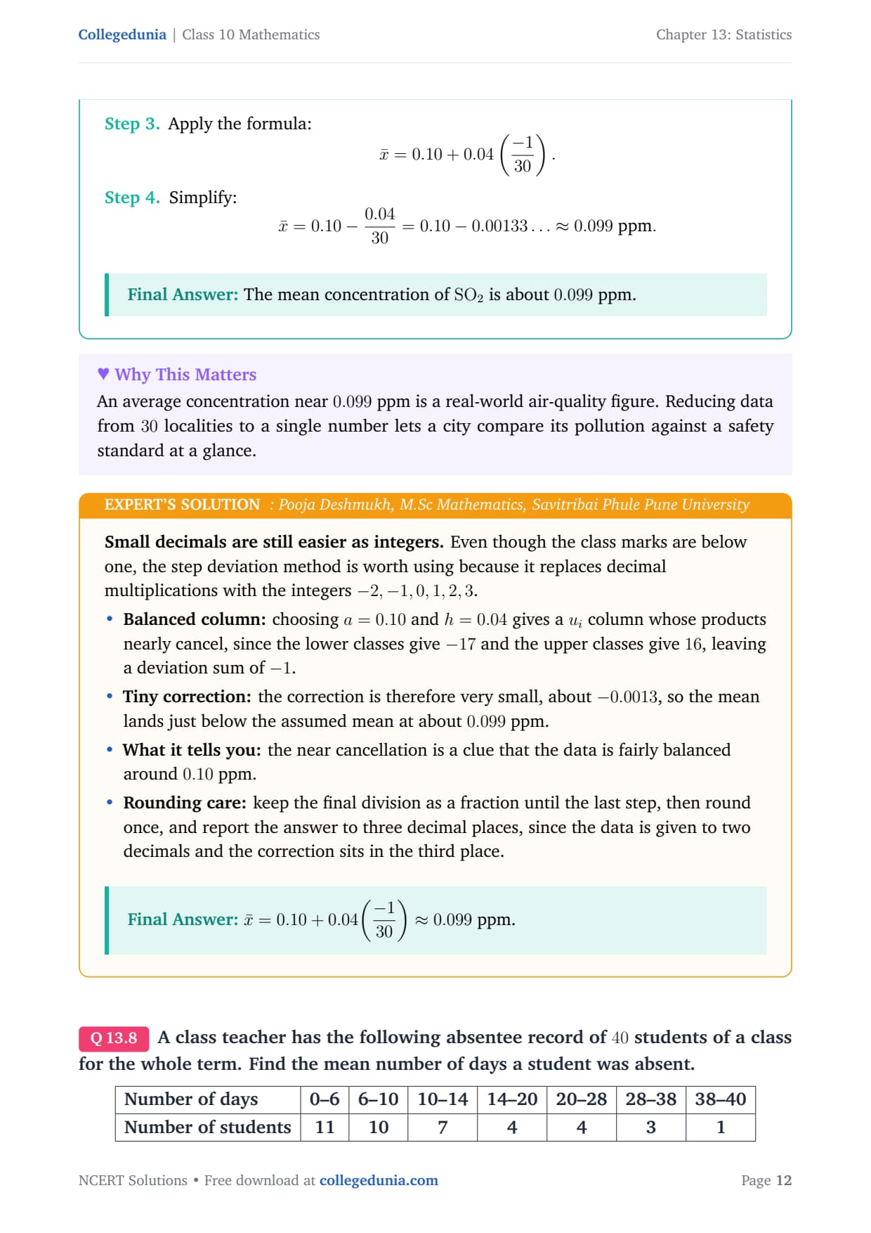
Small decimals are still easier as integers. Even though the class
marks are below one, the step deviation method is worth using because it
replaces decimal multiplications with the integers -2,-1,0,1,2,3.
Balanced column: choosing a=0.10 and h=0.04 gives a
ui column whose products nearly cancel, since the lower classes
give -17 and the upper classes give 16, leaving a deviation sum
of -1.
Tiny correction: the correction is therefore very small,
about -0.0013, so the mean lands just below the assumed mean at
about 0.099 ppm.
What it tells you: the near cancellation is a clue that the
data is fairly balanced around 0.10 ppm.
Rounding care: keep the final division as a fraction until
the last step, then round once, and report the answer to three
decimal places, since the data is given to two decimals and the
correction sits in the third place.
x̄=0.10+0.04(-130)≈ 0.099 ppm.
Q 13.8
A class teacher has the following absentee record of 40
students of a class for the whole term. Find the mean number of days a
student was absent.
tabular|l|c|c|c|c|c|c|c|
Number of days & 0–6 & 6–10 & 10–14 & 14–20 & 20–28 & 28–38 & 38–40
Number of students & 11 & 10 & 7 & 4 & 4 & 3 & 1
tabular
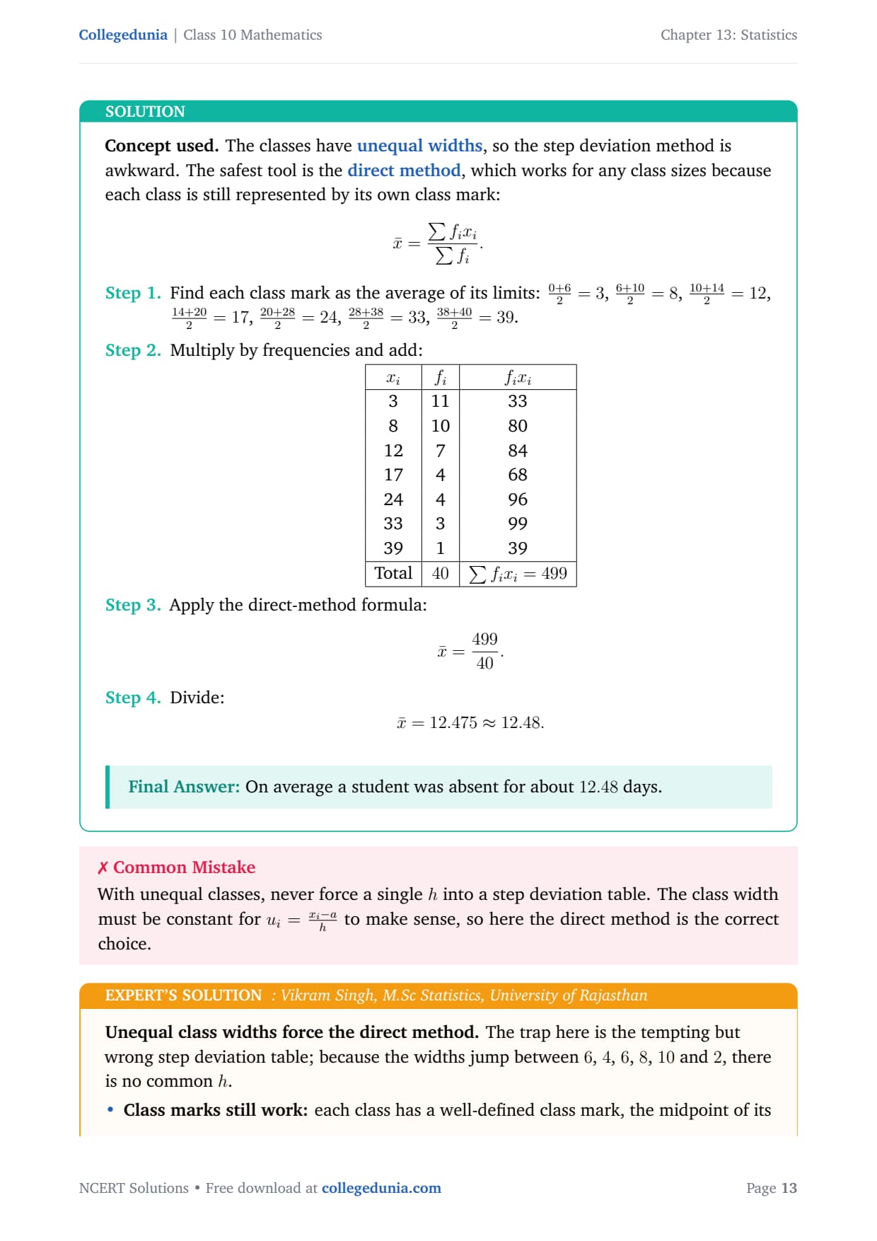
Concept used. The classes have unequal widths, so the
step deviation method is awkward. The safest tool is the direct
method, which works for any class sizes because each class is still
represented by its own class mark:
x̄=∑ fi xi∑ fi.
Find each class mark as the average of its limits:
0+62=3, 6+102=8, 10+142=12,
14+202=17, 20+282=24, 28+382=33,
38+402=39.
Multiply by frequencies and add:
tabular|c|c|c|
xi & fi & fi xi
3 & 11 & 33
8 & 10 & 80
12 & 7 & 84
17 & 4 & 68
24 & 4 & 96
33 & 3 & 99
39 & 1 & 39
Total & 40 & ∑ fi xi=499
tabular
Apply the direct-method formula:
x̄=49940.
Divide:
x̄=12.475≈ 12.48.
On average a student was absent for about 12.48 days.
VS
Vikram Singh
M.Sc Statistics, University of Rajasthan
Verified Expert
Unequal class widths force the direct method. The trap here is the
tempting but wrong step deviation table; because the widths jump between 6,
4, 6, 8, 10 and 2, there is no common h.
Class marks still work: each class has a well-defined class
mark, the midpoint of its own limits, even when the widths differ, so
the direct method handles them all.
The arithmetic: the products fi xi sum to 499, and
dividing by the 40 students gives 12.475, which rounds to 12.48
days.
Why it is low: the mean sits well below the upper classes
because most students, 21 of the 40, fall in the two lowest
absence bands.
Checkpoint and reasoning: the mean must lie between the
smallest class mark 3 and the largest 39, and 12.48 does, so
state explicitly that the unequal classes are why the direct method
is used, because an examiner rewards the reasoning not just the
number.
x̄=49940=12.475≈ 12.48 days.
Q 13.9
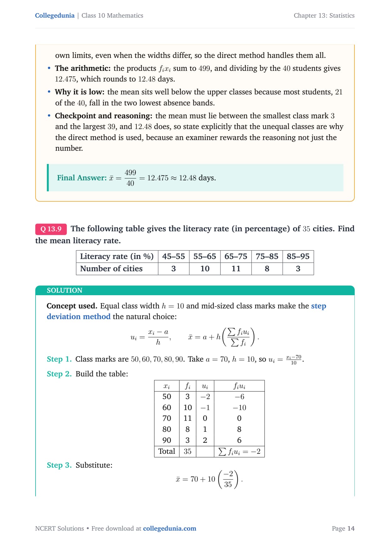
The following table gives the literacy rate (in percentage) of
35 cities. Find the mean literacy rate.
tabular|l|c|c|c|c|c|
Literacy rate (in %) & 45–55 & 55–65 & 65–75 & 75–85 & 85–95
Number of cities & 3 & 10 & 11 & 8 & 3
tabular
Concept used. Equal class width h=10 and mid-sized class marks
make the step deviation method the natural choice:
ui=xi-ah, x̄=a+h(∑ fi ui∑ fi).
Class marks are 50,60,70,80,90. Take a=70, h=10, so
ui=xi-7010.
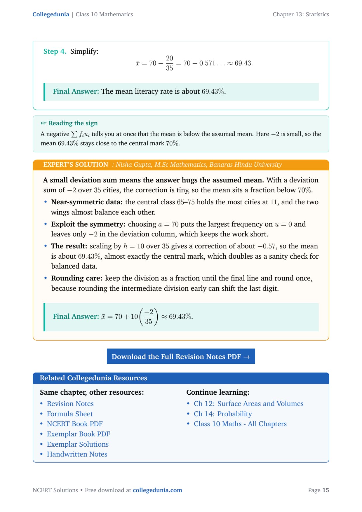
A small deviation sum means the answer hugs the assumed mean. With
a deviation sum of -2 over 35 cities, the correction is tiny, so the
mean sits a fraction below 70%.
Near-symmetric data: the central class 65–75 holds the
most cities at 11, and the two wings almost balance each other.
Exploit the symmetry: choosing a=70 puts the largest
frequency on u=0 and leaves only -2 in the deviation column,
which keeps the work short.
The result: scaling by h=10 over 35 gives a correction
of about -0.57, so the mean is about 69.43%, almost exactly the
central mark, which doubles as a sanity check for balanced data.
Rounding care: keep the division as a fraction until the
final line and round once, because rounding the intermediate division
early can shift the last digit.
x̄=70+10(-235)≈ 69.43%.
NCERT solutions Class 10 Mathematics Chapter 13 Statistics
All 6 questions with collapsible Solution and Expert Solution. Tap a button to reveal the working.
Exercise 13.2
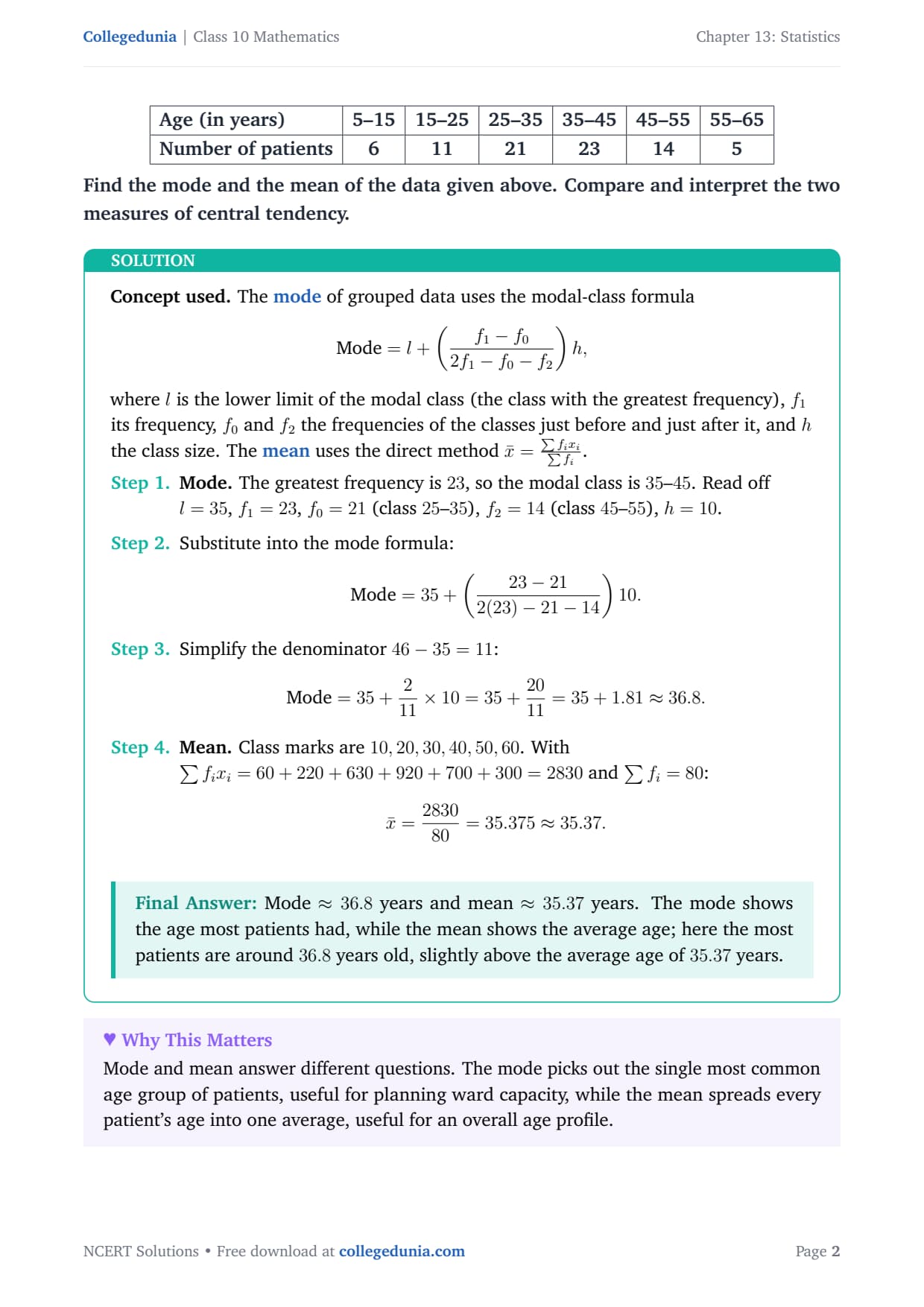
Q 13.1
The following table shows the ages of the patients admitted in
a hospital during a year:
tabular|l|c|c|c|c|c|c|
Age (in years) & 5–15 & 15–25 & 25–35 & 35–45 & 45–55 & 55–65
Number of patients & 6 & 11 & 21 & 23 & 14 & 5
tabular
Find the mode and the mean of the data given above. Compare and interpret
the two measures of central tendency.
Concept used. The mode of grouped data uses the
modal-class formula
Mode=l+(f1-f02f1-f0-f2)h,
where l is the lower limit of the modal class (the class with the
greatest frequency), f1 its frequency, f0 and f2 the frequencies
of the classes just before and just after it, and h the class size. The
mean uses the direct method
x̄=∑ fi xi∑ fi.
Mode. The greatest frequency is 23, so the modal class
is 35–45. Read off l=35, f1=23, f0=21 (class
25–35), f2=14 (class 45–55), h=10.
Substitute into the mode formula:
Mode=35+(23-212(23)-21-14)10.
Simplify the denominator 46-35=11:
Mode=35+211× 10=35+2011=35+1.81≈ 36.8.
Mean. Class marks are 10,20,30,40,50,60. With
∑ fi xi = 60+220+630+920+700+300=2830 and
∑ fi = 80:
x̄=283080=35.375≈ 35.37.
Mode ≈ 36.8 years and mean ≈ 35.37 years. The mode shows the age most patients had, while the mean shows the average age; here the most patients are around 36.8 years old, slightly above the average age of 35.37 years.
SM
Shalini Menon
M.Sc Statistics, University of Hyderabad
Verified Expert
Two measures, two different stories about the same patients. The
mode comes from one class only, while the mean uses all six, which is exactly
why they differ.
Mode reasoning: spotting the modal class is the whole
battle, and 35–45 carries the top frequency 23 with neighbours
21 and 14; the small numerator over a moderate denominator pushes
the mode only about 1.8 above the lower limit, giving 36.8 years.
Mean reasoning: the products fi xi total 2830 over the
80 patients, giving an average age of about 35.37 years.
What the gap shows: the two numbers being close, with the
mode just above the mean, tells you the age distribution is roughly
symmetric with a slight bunching near 40 years.
Interpretation mark: write one comparison sentence saying
the most frequent age is about 36.8 while the average is about
35.4; quoting the numbers without that sentence usually loses the
interpretation mark.
Mode ≈ 36.8 years, mean ≈ 35.37 years; the most common age is a little above the average age.
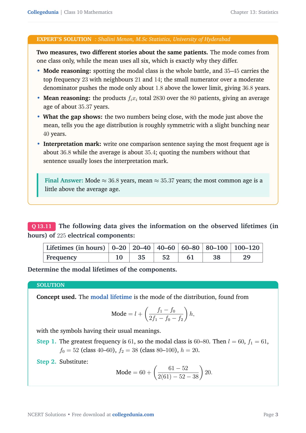
Q 13.2
The following data gives the information on the observed
lifetimes (in hours) of 225 electrical components:
Concept used. The modal lifetime is the mode of the
distribution, found from
Mode=l+(f1-f02f1-f0-f2)h,
with the symbols having their usual meanings.
The greatest frequency is 61, so the modal class is 60–80.
Then l=60, f1=61, f0=52 (class 40–60), f2=38
(class 80–100), h=20.
Substitute:
Mode=60+(61-522(61)-52-38)20.
Simplify the denominator 122-90=32:
Mode=60+932× 20.
Finish the arithmetic:
Mode=60+18032=60+5.625=65.625.
The modal lifetime of the components is 65.625 hours.
HK
Harish Kumar
M.Sc Mathematics, University of Calcutta
Verified Expert
Lock the three frequencies to their positions, then it is one
substitution. The only place students lose marks here is swapping f0 and
f2, so fix them by position before touching the formula.
Fix by position: the modal class 60–80 has f1=61;
the class immediately before gives f0=52 and the class
immediately after gives f2=38, never the other way round.
One substitution: the numerator 9 and the denominator
32 are both straightforward, so the mode comes out as 65.625
hours in a single step.
Why it sits there: the answer landing a quarter of the way
up from 60 is exactly what the formula should give, since the
modal frequency is much closer to the class after than the class
before.
Avoid the swap: label the three frequencies above their
numbers in the substitution, which is the surest way to prevent the
common swap error and to show the examiner your reasoning.
Mode=60+932× 20=65.625 hours.
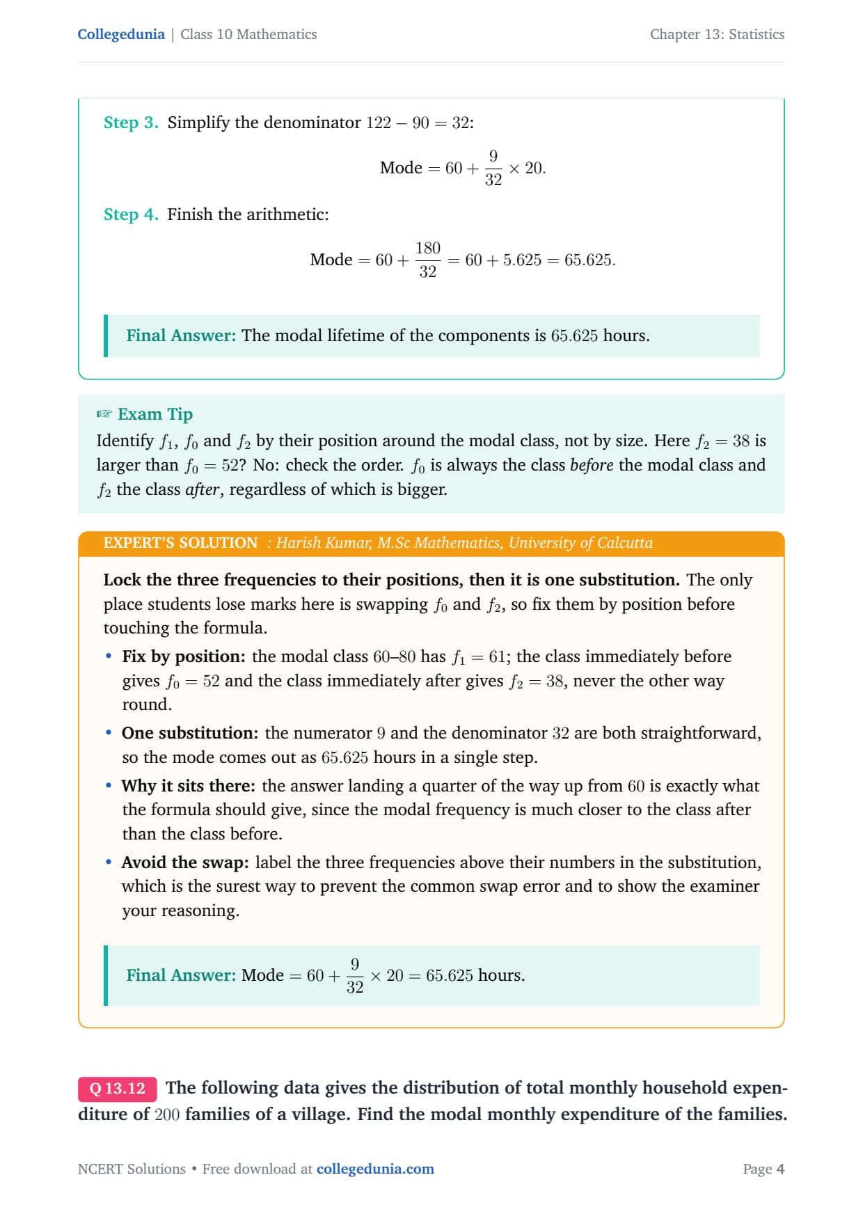
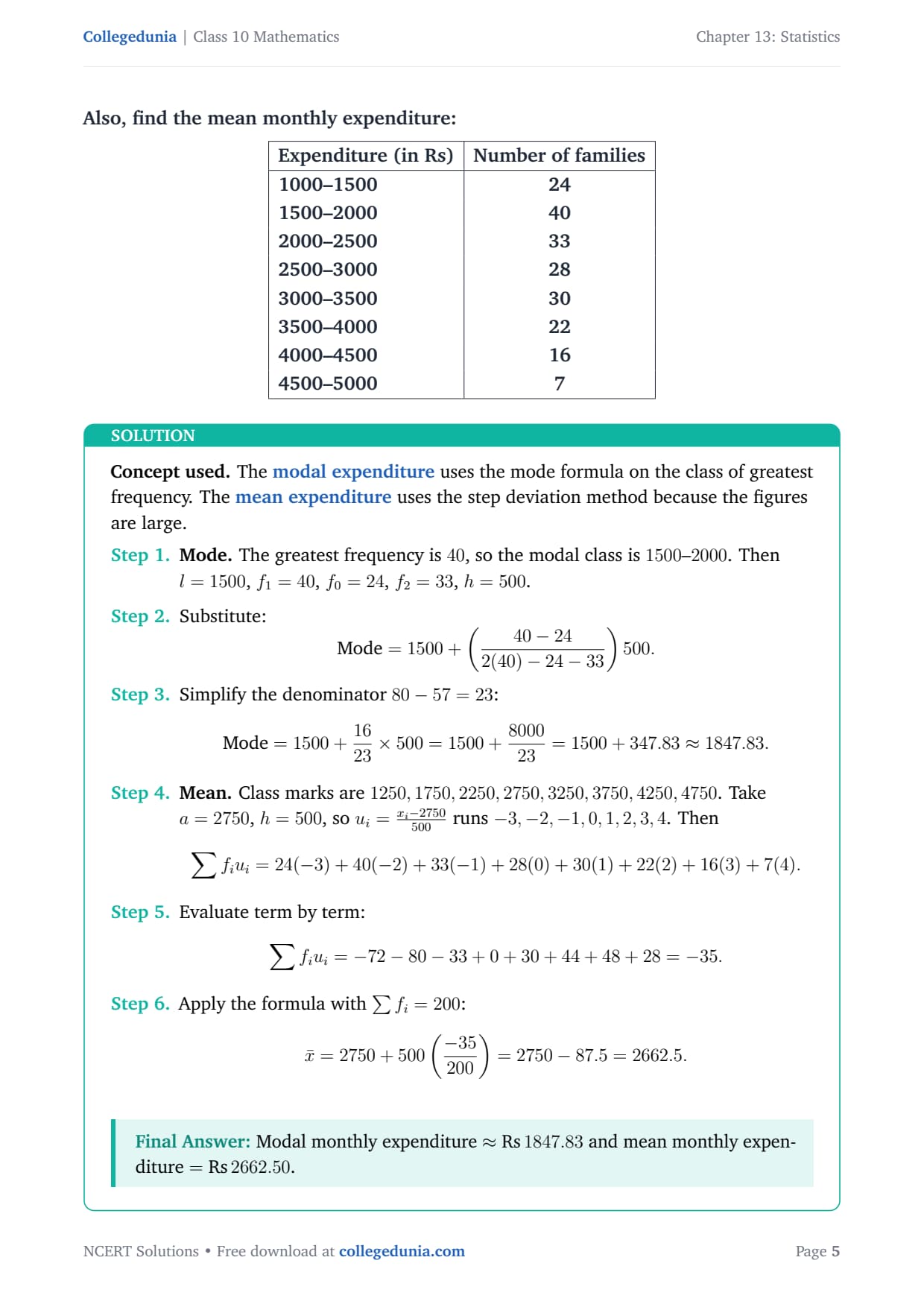
Q 13.3
The following data gives the distribution of total monthly
household expenditure of 200 families of a village. Find the modal
monthly expenditure of the families. Also, find the mean monthly
expenditure:
Concept used. The modal expenditure uses the mode
formula on the class of greatest frequency. The mean
expenditure uses the step deviation method because the figures are
large.
Mode. The greatest frequency is 40, so the modal class
is 1500–2000. Then l=1500, f1=40, f0=24, f2=33,
h=500.
Substitute:
Mode=1500+(40-242(40)-24-33)500.
Simplify the denominator 80-57=23:
Mode=1500+1623× 500=1500+800023=1500+347.83≈ 1847.83.
Mean. Class marks are 1250,1750,2250,2750,3250,3750,
4250,4750. Take a=2750, h=500, so
ui=xi-2750500 runs -3,-2,-1,0,1,2,3,4. Then
∑ fi ui = 24(-3)+40(-2)+33(-1)+28(0)+30(1)+22(2)+16(3)+7(4).
Evaluate term by term:
∑ fi ui=-72-80-33+0+30+44+48+28=-35.
Apply the formula with ∑ fi=200:
x̄=2750+500(-35200)=2750-87.5=2662.5.
Modal monthly expenditure ≈1847.83 and mean monthly expenditure =2662.50.
RA
Ritu Agarwal
M.Sc Statistics, University of Lucknow
Verified Expert
Mode reads one class, mean reads all eight. The contrast here is
striking: the mode at about 1848 rupees is far below the mean at 2662.50
rupees, and that gap is the real lesson.
Mode: the modal class 1500–2000 has the top frequency
40 with neighbours 24 and 33, which places the mode at about
1847.83 rupees.
Mean: choosing a=2750 keeps the ui values in the range
-3 to 4; the deviation column sums to -35, and scaling gives a
correction of -87.5, so the mean is 2662.50 rupees.
Read the skew: the mode being far below the mean signals a
right-skewed distribution, where most families cluster at lower
expenditure but a tail of higher-spending families pulls the average
up.
Full marks: recognising that skew and saying so in words is
what distinguishes a complete answer from one that just lists the two
numbers.
Mode ≈1847.83; mean =2662.50 (data is right-skewed).
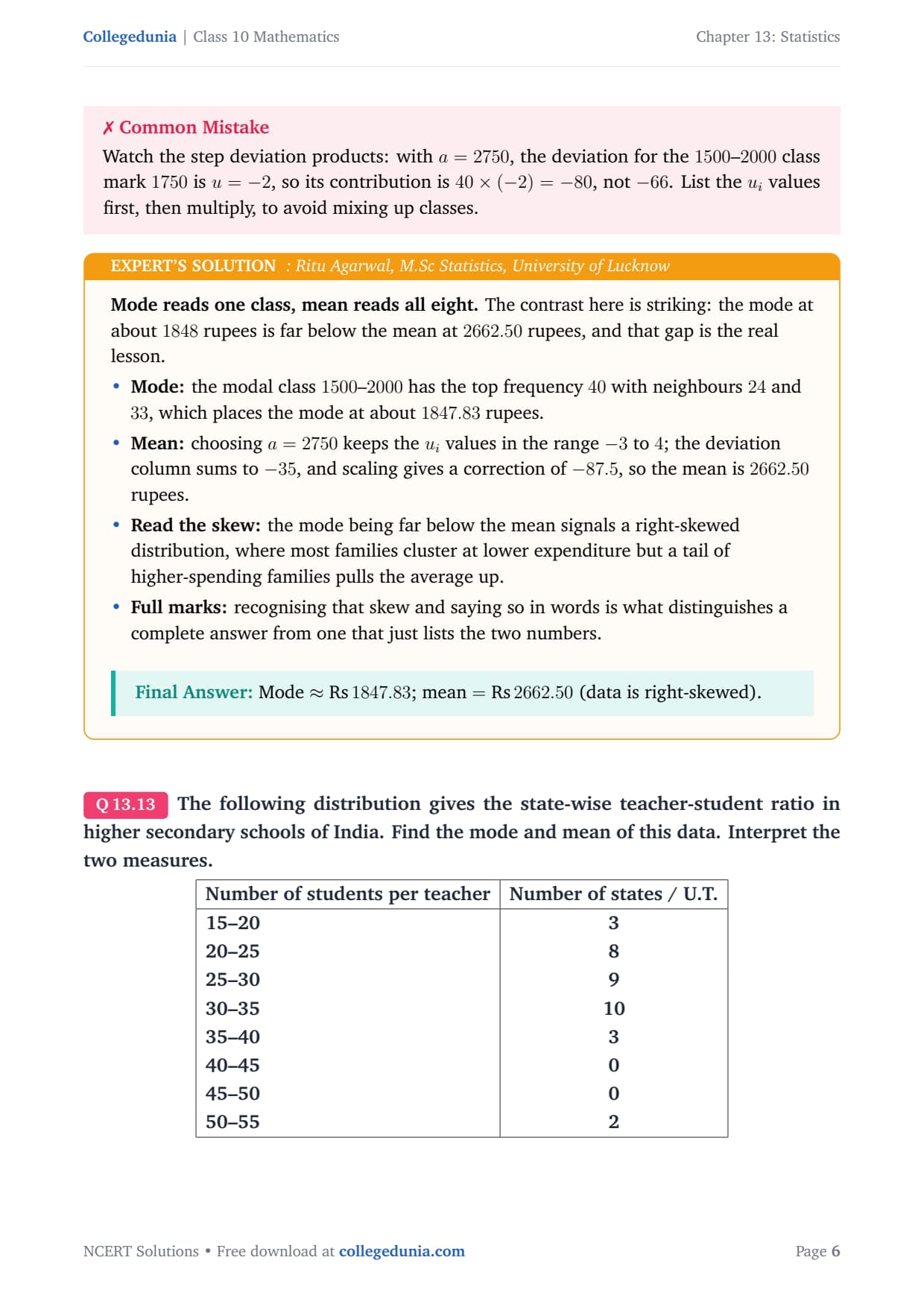
Q 13.4
The following distribution gives the state-wise teacher-student
ratio in higher secondary schools of India. Find the mode and mean of
this data. Interpret the two measures.
tabular|l|c|
Number of students per teacher & Number of states / U.T.
15–20 & 3
20–25 & 8
25–30 & 9
30–35 & 10
35–40 & 3
40–45 & 0
45–50 & 0
50–55 & 2
tabular
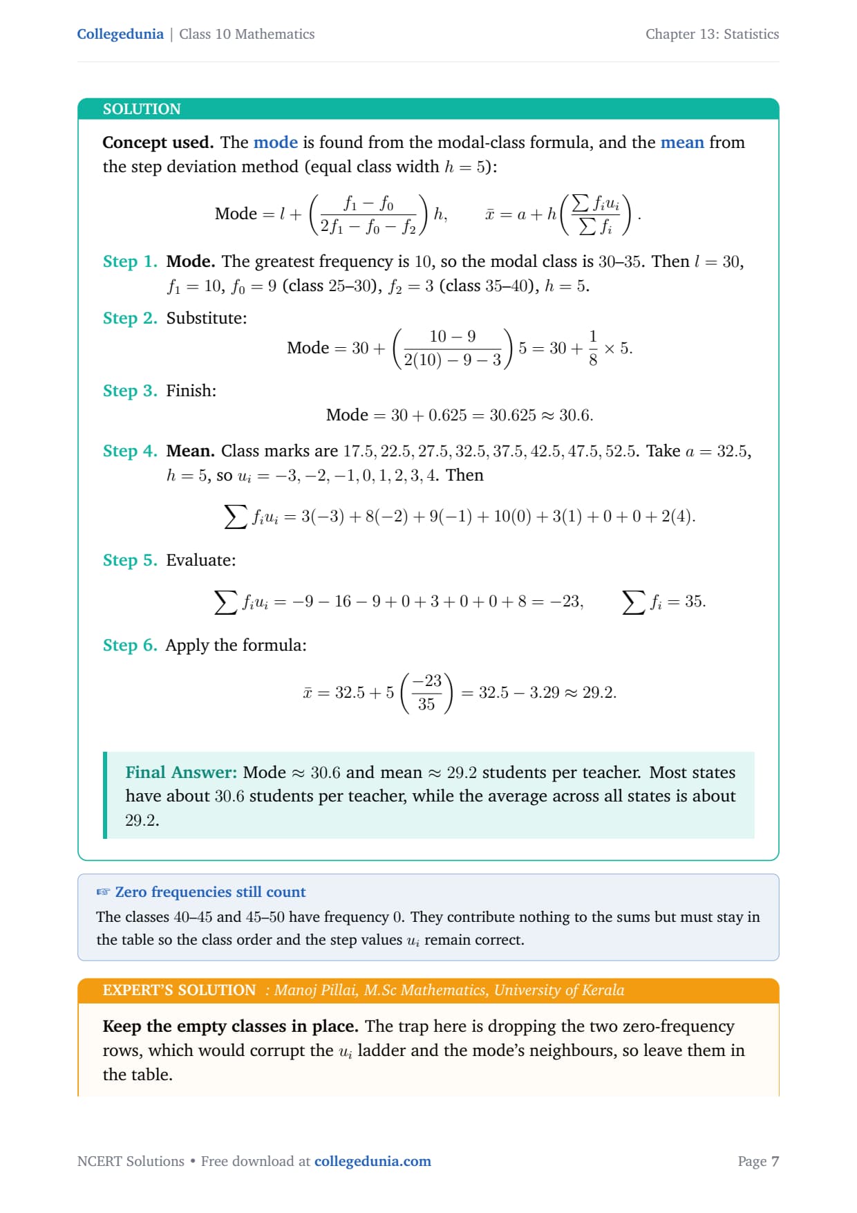
Concept used. The mode is found from the modal-class
formula, and the mean from the step deviation method (equal
class width h=5):
Mode=l+(f1-f02f1-f0-f2)h, x̄=a+h(∑ fi ui∑ fi).
Mode. The greatest frequency is 10, so the modal class
is 30–35. Then l=30, f1=10, f0=9 (class 25–30),
f2=3 (class 35–40), h=5.
Substitute:
Mode=30+(10-92(10)-9-3)5=30+18× 5.
Finish:
Mode=30+0.625=30.625≈ 30.6.
Mean. Class marks are 17.5,22.5,27.5,32.5,37.5,42.5,
47.5,52.5. Take a=32.5, h=5, so ui=-3,-2,-1,0,1,2,3,4.
Then
∑ fi ui = 3(-3)+8(-2)+9(-1)+10(0)+3(1)+0+0+2(4).
Evaluate:
∑ fi ui=-9-16-9+0+3+0+0+8=-23, ∑ fi=35.
Apply the formula:
x̄=32.5+5(-2335)=32.5-3.29≈ 29.2.
Mode ≈ 30.6 and mean ≈ 29.2 students per teacher. Most states have about 30.6 students per teacher, while the average across all states is about 29.2.
MP
Manoj Pillai
M.Sc Mathematics, University of Kerala
Verified Expert
Keep the empty classes in place. The trap here is dropping the two
zero-frequency rows, which would corrupt the ui ladder and the mode's
neighbours, so leave them in the table.
Mode: the modal class 30–35 has f1=10 with
neighbours 9 and 3; the small numerator over denominator 8
gives a mode just 0.625 above 30, namely 30.625.
Mean: taking a=32.5 produces a deviation column summing to
-23, and the scaling gives a correction of about -3.29, so the
mean is about 29.2 students per teacher.
Read the shape: the mode being a little above the mean, with
a long thin tail at 50–55, again points to a mild right skew in
the data.
Interpretation: write that a typical state runs at roughly
30 students per teacher while the all-India average is a touch
lower at about 29, the difference coming from the handful of states
with very high ratios.
Mode ≈ 30.6, mean ≈ 29.2 students per teacher.
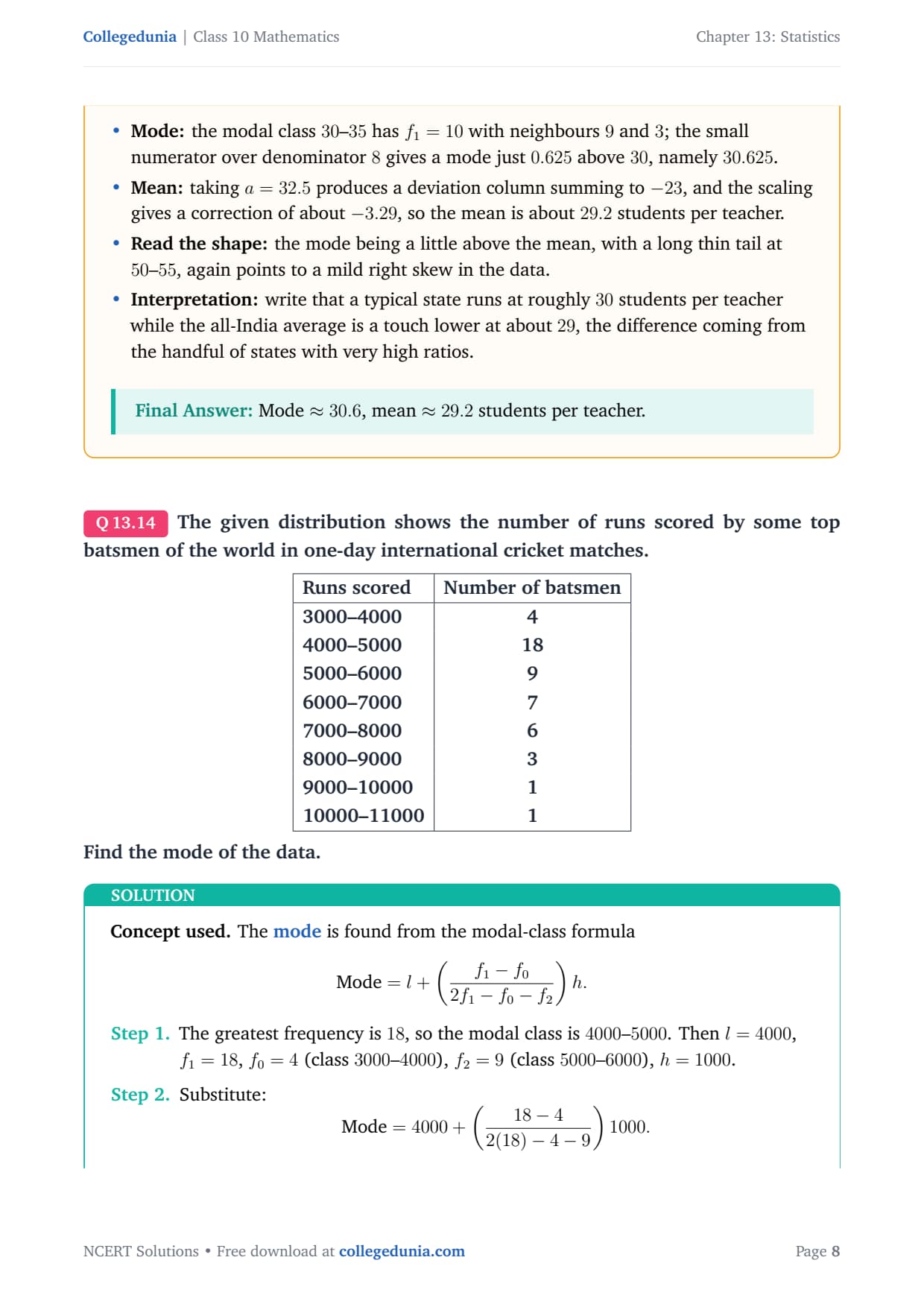
Q 13.5
The given distribution shows the number of runs scored by some
top batsmen of the world in one-day international cricket matches.
Concept used. The mode is found from the modal-class
formula
Mode=l+(f1-f02f1-f0-f2)h.
The greatest frequency is 18, so the modal class is
4000–5000. Then l=4000, f1=18, f0=4 (class
3000–4000), f2=9 (class 5000–6000), h=1000.
Substitute:
Mode=4000+(18-42(18)-4-9)1000.
Simplify the denominator 36-13=23:
Mode=4000+1423× 1000=4000+1400023.
Finish:
Mode=4000+608.7≈ 4608.7.
The mode of the data is about 4608.7 runs.
AR
Arjun Reddy
M.Sc Statistics, University of Hyderabad
Verified Expert
A tall modal class with a low left neighbour pushes the mode well
up. The jump from f0=4 to f1=18 is large, so the mode sits high inside
the modal class.
Big numerator: the numerator 14 is large relative to the
denominator 23, so the fraction is substantial; multiplied by the
big class size h=1000 it adds about 609 runs, giving 4608.7.
Why it sits high: the mode landing more than halfway up the
modal class is the formula's way of saying the data rises steeply
into this class from the sparse band below and falls more gently
afterwards.
Mode is local: only the three frequencies around the modal
class matter, so the long thin tail out to 11000 runs is irrelevant
to the mode, a useful reminder of what the mode measures.
Common slip: write h=1000 explicitly in the substitution,
which avoids the frequent mistake of multiplying the fraction by 1
or by 100 instead of the true class size.
Mode=4000+1423× 1000≈ 4608.7 runs.
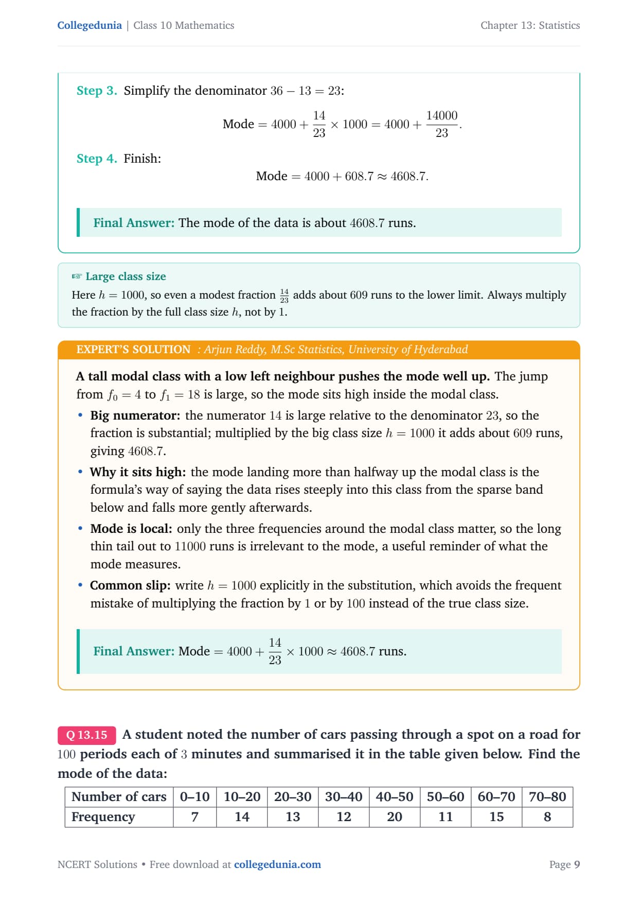
Q 13.6
A student noted the number of cars passing through a spot on a
road for 100 periods each of 3 minutes and summarised it in the table
given below. Find the mode of the data:
Concept used. The mode is found from the modal-class
formula
Mode=l+(f1-f02f1-f0-f2)h.
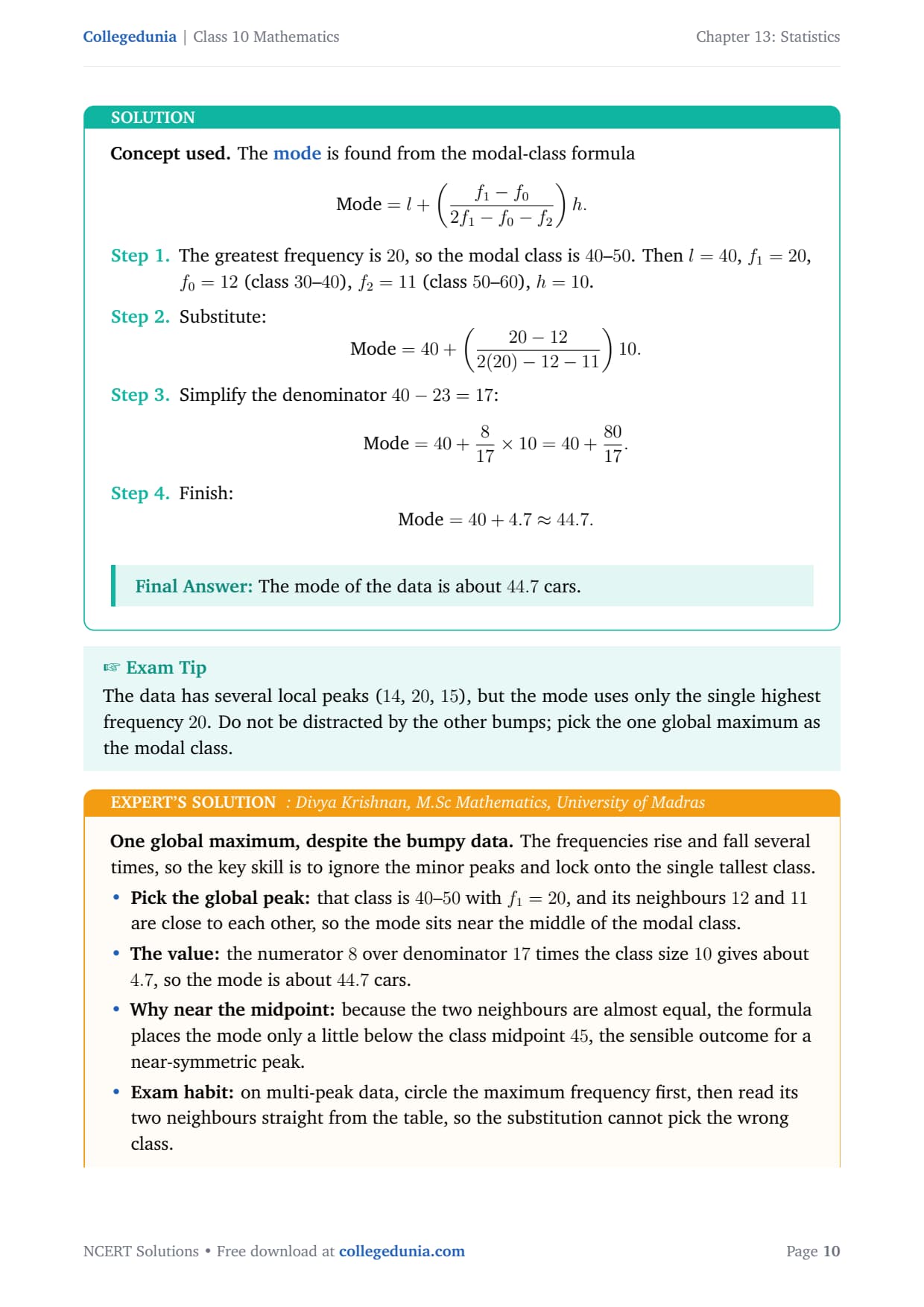
The greatest frequency is 20, so the modal class is 40–50.
Then l=40, f1=20, f0=12 (class 30–40), f2=11
(class 50–60), h=10.
Substitute:
Mode=40+(20-122(20)-12-11)10.
Simplify the denominator 40-23=17:
Mode=40+817× 10=40+8017.
Finish:
Mode=40+4.7≈ 44.7.
The mode of the data is about 44.7 cars.
DK
Divya Krishnan
M.Sc Mathematics, University of Madras
Verified Expert
One global maximum, despite the bumpy data. The frequencies rise
and fall several times, so the key skill is to ignore the minor peaks and
lock onto the single tallest class.
Pick the global peak: that class is 40–50 with
f1=20, and its neighbours 12 and 11 are close to each other,
so the mode sits near the middle of the modal class.
The value: the numerator 8 over denominator 17 times the
class size 10 gives about 4.7, so the mode is about 44.7 cars.
Why near the midpoint: because the two neighbours are almost
equal, the formula places the mode only a little below the class
midpoint 45, the sensible outcome for a near-symmetric peak.
Exam habit: on multi-peak data, circle the maximum frequency
first, then read its two neighbours straight from the table, so the
substitution cannot pick the wrong class.
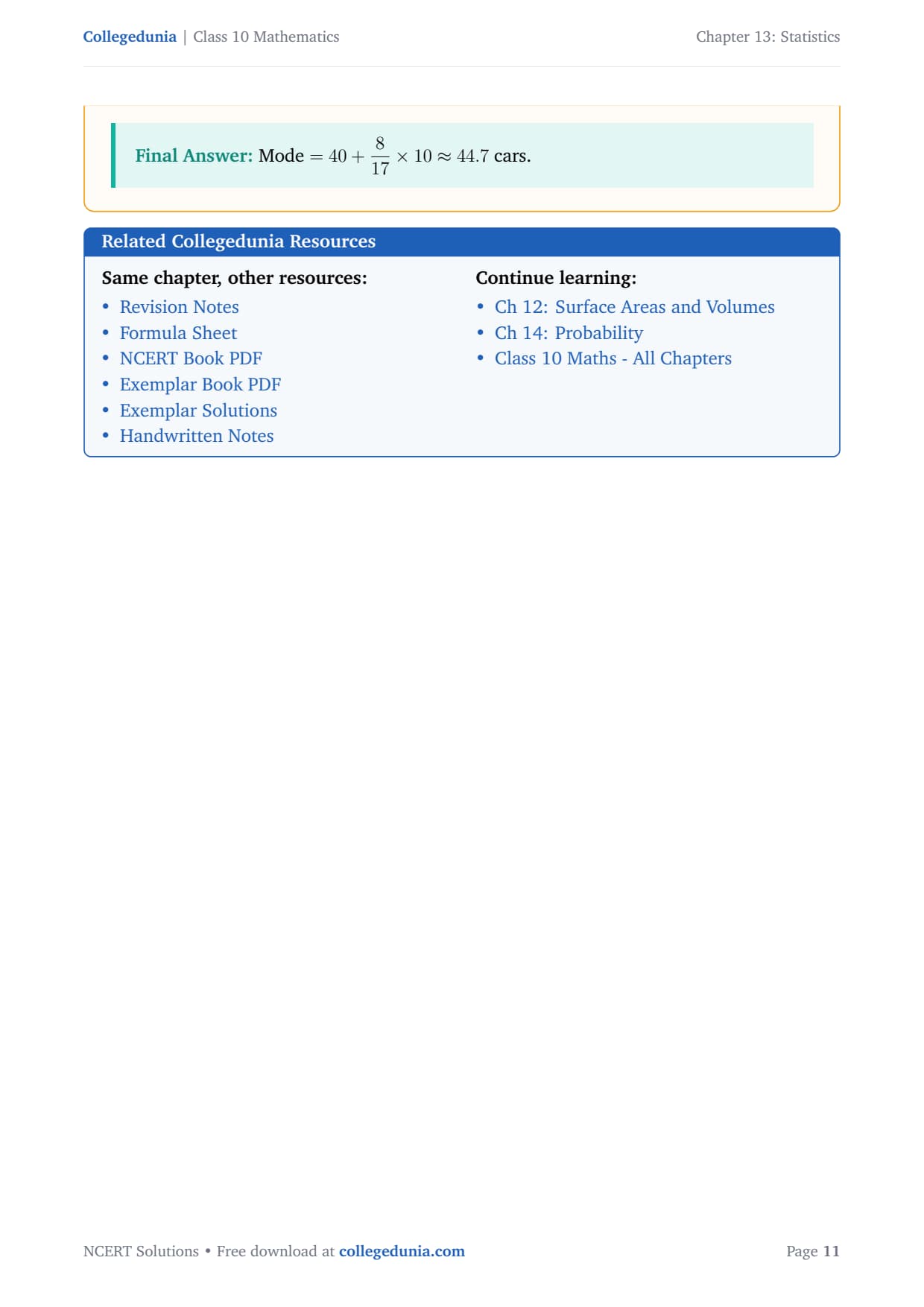
Mode=40+817× 10≈ 44.7 cars.
NCERT solutions Class 10 Mathematics Chapter 13 Statistics
All 7 questions with collapsible Solution and Expert Solution. Tap a button to reveal the working.
Exercise 13.3
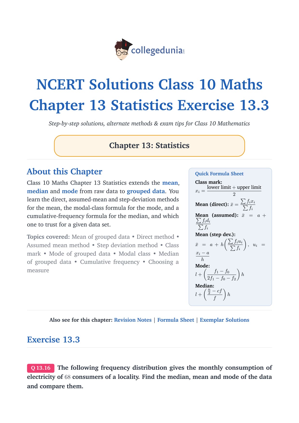
Q 13.1
The following frequency distribution gives the monthly
consumption of electricity of 68 consumers of a locality. Find the
median, mean and mode of the data and compare them.
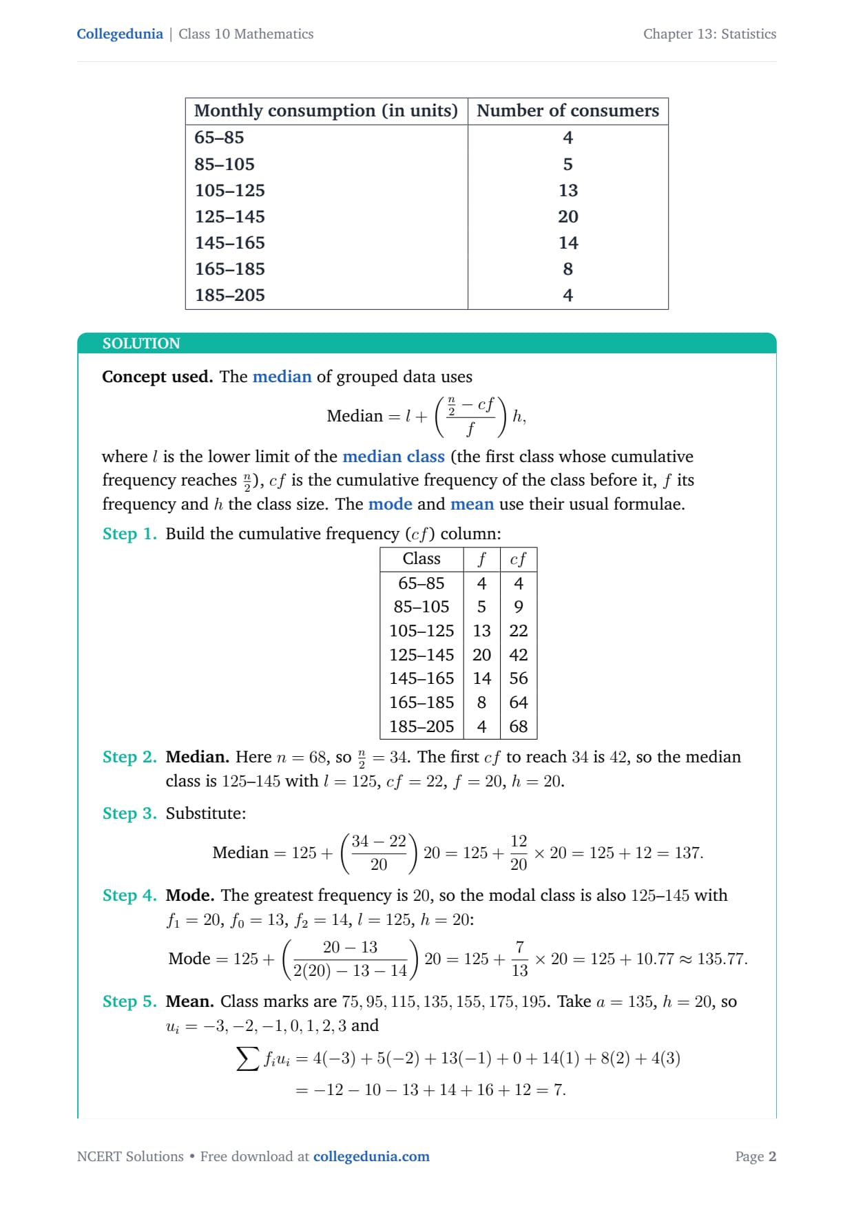
tabular|l|c|
Monthly consumption (in units) & Number of consumers
65–85 & 4
85–105 & 5
105–125 & 13
125–145 & 20
145–165 & 14
165–185 & 8
185–205 & 4
tabular
Concept used. The median of grouped data uses
Median=l+(n2-cff)h,
where l is the lower limit of the median class (the first
class whose cumulative frequency reaches n2), cf is the
cumulative frequency of the class before it, f its frequency and h
the class size. The mode and mean use their usual
formulae.
Mode. The greatest frequency is 20, so the modal class
is also 125–145 with f1=20, f0=13, f2=14, l=125,
h=20:
Mode=125+(20-132(20)-13-14)20=125+713× 20=125+10.77≈ 135.77.
Mean. Class marks are 75,95,115,135,155,175,195. Take
a=135, h=20, so ui=-3,-2,-1,0,1,2,3 and
MATH0
Then
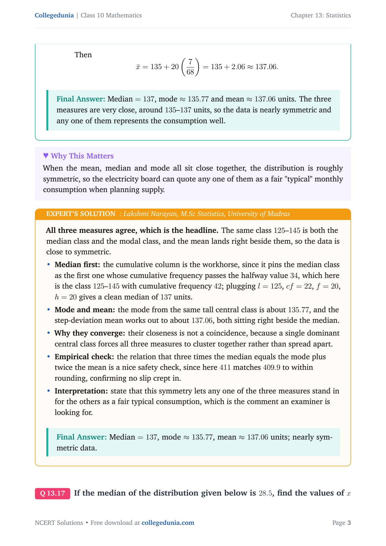
x̄=135+20(768)=135+2.06≈ 137.06.
Median =137, mode ≈ 135.77 and mean ≈ 137.06 units. The three measures are very close, around 135–137 units, so the data is nearly symmetric and any one of them represents the consumption well.
LN
Lakshmi Narayan
M.Sc Statistics, University of Madras
Verified Expert
All three measures agree, which is the headline. The same class
125–145 is both the median class and the modal class, and the mean lands
right beside them, so the data is close to symmetric.
Median first: the cumulative column is the workhorse, since
it pins the median class as the first one whose cumulative frequency
passes the halfway value 34, which here is the class 125–145
with cumulative frequency 42; plugging l=125, cf=22, f=20,
h=20 gives a clean median of 137 units.
Mode and mean: the mode from the same tall central class is
about 135.77, and the step-deviation mean works out to about
137.06, both sitting right beside the median.
Why they converge: their closeness is not a coincidence,
because a single dominant central class forces all three measures to
cluster together rather than spread apart.
Empirical check: the relation that three times the median
equals the mode plus twice the mean is a nice safety check, since
here 411 matches 409.9 to within rounding, confirming no slip
crept in.
Interpretation: state that this symmetry lets any one of the
three measures stand in for the others as a fair typical consumption,
which is the comment an examiner is looking for.
Median =137, mode ≈ 135.77, mean ≈ 137.06 units; nearly symmetric data.
Q 13.2
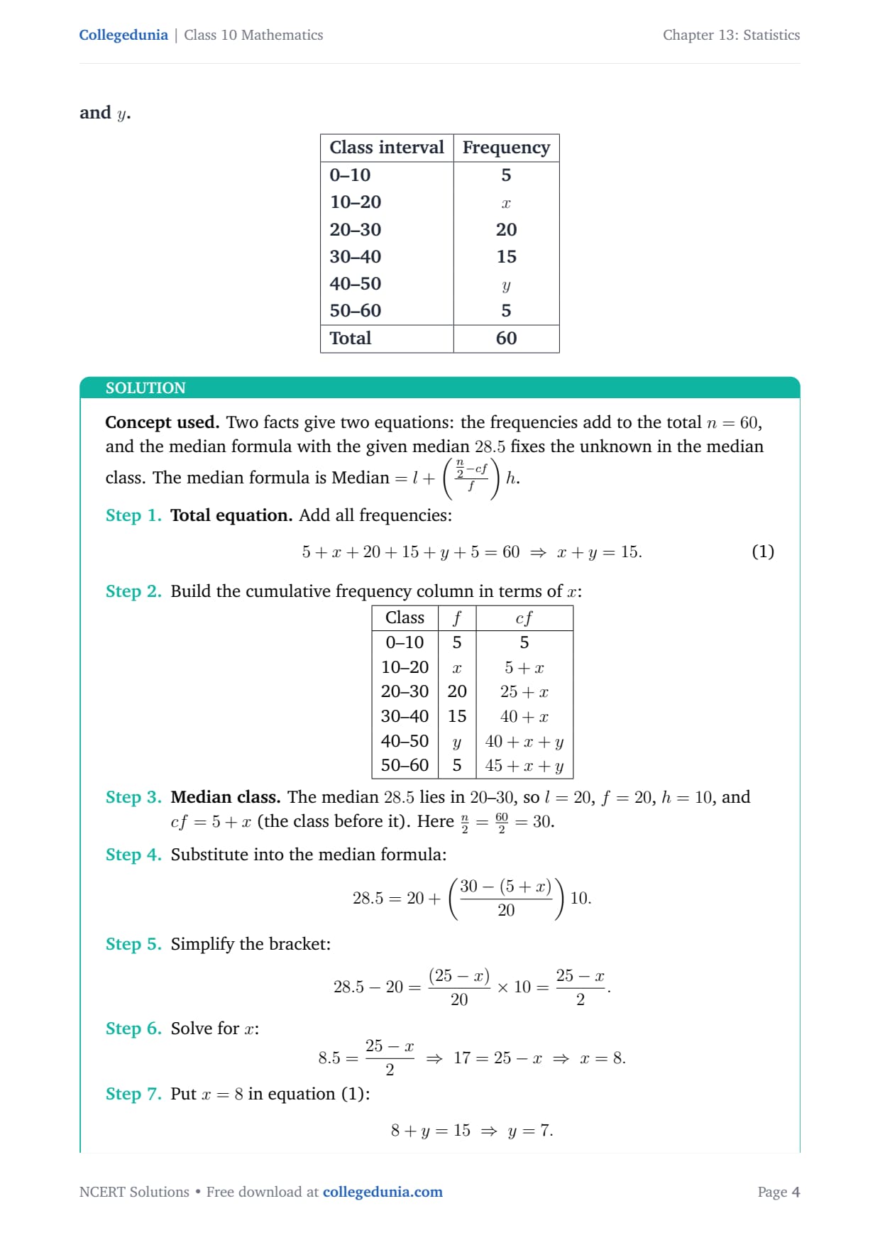
If the median of the distribution given below is 28.5, find
the values of x and y.
tabular|l|c|
Class interval & Frequency
0–10 & 5
10–20 & x
20–30 & 20
30–40 & 15
40–50 & y
50–60 & 5
Total & 60
tabular
Concept used. Two facts give two equations: the frequencies add
to the total n=60, and the median formula with the given median 28.5
fixes the unknown in the median class. The median formula is
Median=l+(n2-cff)h.
Total equation. Add all frequencies:
5+x+20+15+y+5=60 ⇒ x+y=15. 1
Build the cumulative frequency column in terms of x:
tabular|c|c|c|
Class & f & cf
0–10 & 5 & 5
10–20 & x & 5+x
20–30 & 20 & 25+x
30–40 & 15 & 40+x
40–50 & y & 40+x+y
50–60 & 5 & 45+x+y
tabular
Median class. The median 28.5 lies in 20–30, so
l=20, f=20, h=10, and cf=5+x (the class before it). Here
n2=602=30.
Substitute into the median formula:
28.5=20+(30-(5+x)20)10.
Simplify the bracket:
28.5-20=(25-x)20× 10=25-x2.
Solve for x:
8.5=25-x2 ⇒ 17=25-x ⇒ x=8.
Put x=8 in equation (1):
8+y=15 ⇒ y=7.
x=8 and y=7.
FA
Farhan Ali
M.Sc Mathematics, Aligarh Muslim University
Verified Expert
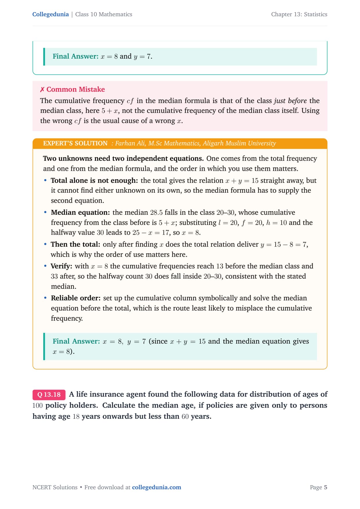
Two unknowns need two independent equations. One comes from the
total frequency and one from the median formula, and the order in which you
use them matters.
Total alone is not enough: the total gives the relation
x+y=15 straight away, but it cannot find either unknown on its own,
so the median formula has to supply the second equation.
Median equation: the median 28.5 falls in the class
20–30, whose cumulative frequency from the class before is
5+x; substituting l=20, f=20, h=10 and the halfway value 30
leads to 25-x=17, so x=8.
Then the total: only after finding x does the total
relation deliver y=15-8=7, which is why the order of use matters
here.
Verify: with x=8 the cumulative frequencies reach 13
before the median class and 33 after, so the halfway count 30
does fall inside 20–30, consistent with the stated median.
Reliable order: set up the cumulative column symbolically
and solve the median equation before the total, which is the route
least likely to misplace the cumulative frequency.
x=8, y=7 (since x+y=15 and the median equation gives x=8).
Q 13.3
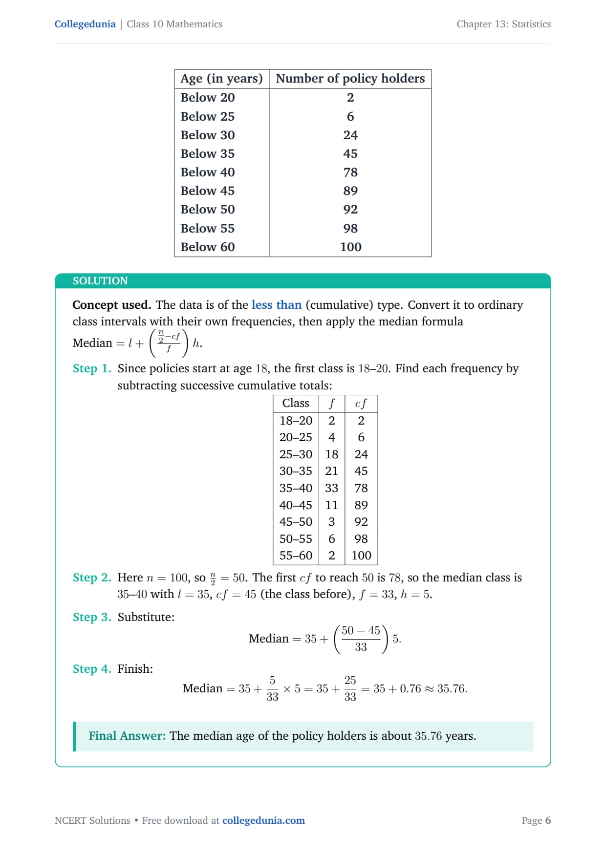
A life insurance agent found the following data for
distribution of ages of 100 policy holders. Calculate the median age,
if policies are given only to persons having age 18 years onwards but
less than 60 years.
Concept used. The data is of the less than (cumulative)
type. Convert it to ordinary class intervals with their own frequencies,
then apply the median formula
Median=l+(n2-cff)h.
Since policies start at age 18, the first class is 18–20.
Find each frequency by subtracting successive cumulative totals:
Here n=100, so n2=50. The first cf to reach 50
is 78, so the median class is 35–40 with l=35, cf=45
(the class before), f=33, h=5.
Substitute:
Median=35+(50-4533)5.
Finish:
Median=35+533× 5=35+2533=35+0.76≈ 35.76.
The median age of the policy holders is about 35.76 years.
SJ
Sunita Joshi
M.Sc Statistics, University of Pune
Verified Expert
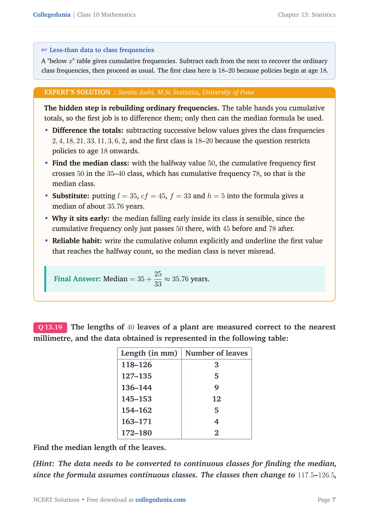
The hidden step is rebuilding ordinary frequencies. The table hands
you cumulative totals, so the first job is to difference them; only then can
the median formula be used.
Difference the totals: subtracting successive below values
gives the class frequencies 2, 4, 18, 21, 33, 11, 3, 6, 2, and the
first class is 18–20 because the question restricts policies to
age 18 onwards.
Find the median class: with the halfway value 50, the
cumulative frequency first crosses 50 in the 35–40 class,
which has cumulative frequency 78, so that is the median class.
Substitute: putting l=35, cf=45, f=33 and h=5 into
the formula gives a median of about 35.76 years.
Why it sits early: the median falling early inside its class
is sensible, since the cumulative frequency only just passes 50
there, with 45 before and 78 after.
Reliable habit: write the cumulative column explicitly and
underline the first value that reaches the halfway count, so the
median class is never misread.
Median=35+2533≈ 35.76 years.
Q 13.4
The lengths of 40 leaves of a plant are measured correct to
the nearest millimetre, and the data obtained is represented in the
following table:
tabular|l|c|
Length (in mm) & Number of leaves
118–126 & 3
127–135 & 5
136–144 & 9
145–153 & 12
154–162 & 5
163–171 & 4
172–180 & 2
tabular
Find the median length of the leaves.
(Hint: The data needs to be converted to continuous classes for
finding the median, since the formula assumes continuous classes. The
classes then change to 117.5–126.5, 126.5–135.5, ,
171.5–180.5.)
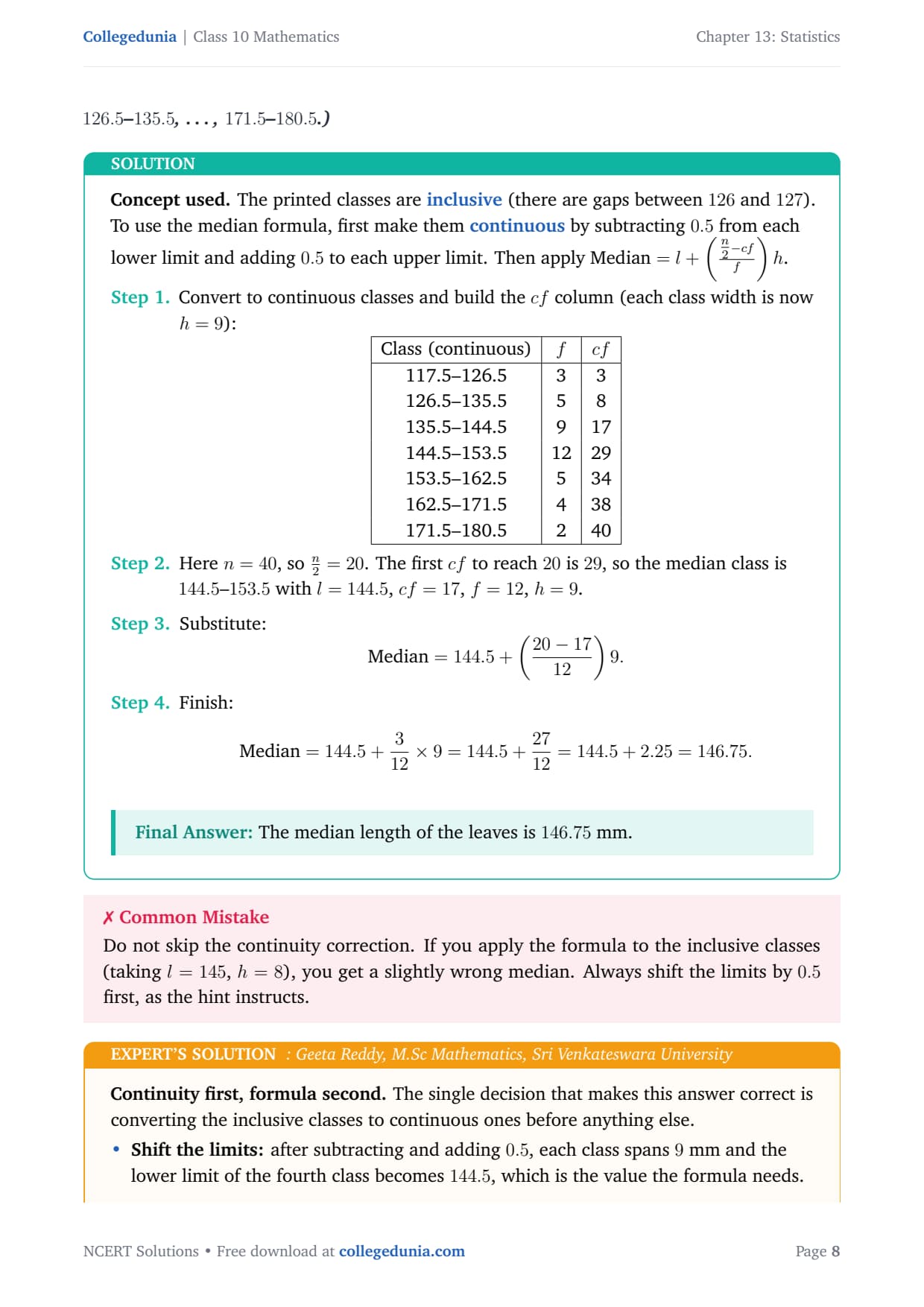
Concept used. The printed classes are inclusive
(there are gaps between 126 and 127). To use the median formula,
first make them continuous by subtracting 0.5 from each lower
limit and adding 0.5 to each upper limit. Then apply
Median=l+(n2-cff)h.
Convert to continuous classes and build the cf column (each
class width is now h=9):
Continuity first, formula second. The single decision that makes
this answer correct is converting the inclusive classes to continuous ones
before anything else.
Shift the limits: after subtracting and adding 0.5, each
class spans 9 mm and the lower limit of the fourth class becomes
144.5, which is the value the formula needs.
Locate the median class: the cumulative column reaches 17
before the median class and 29 at its end, so with the halfway
value 20 the median class is 144.5–153.5.
Substitute: putting l=144.5, cf=17, f=12 and h=9
into the formula gives a median length of 146.75 mm.
Why a quarter in: the median landing a quarter of the way
into the class fits the fact that only 3 of the 12 leaves there
are needed to pass the halfway mark.
Presentation: show the converted class column alongside the
original, so the examiner sees the continuity correction was applied
deliberately rather than by accident.
Median=144.5+2712=146.75 mm.
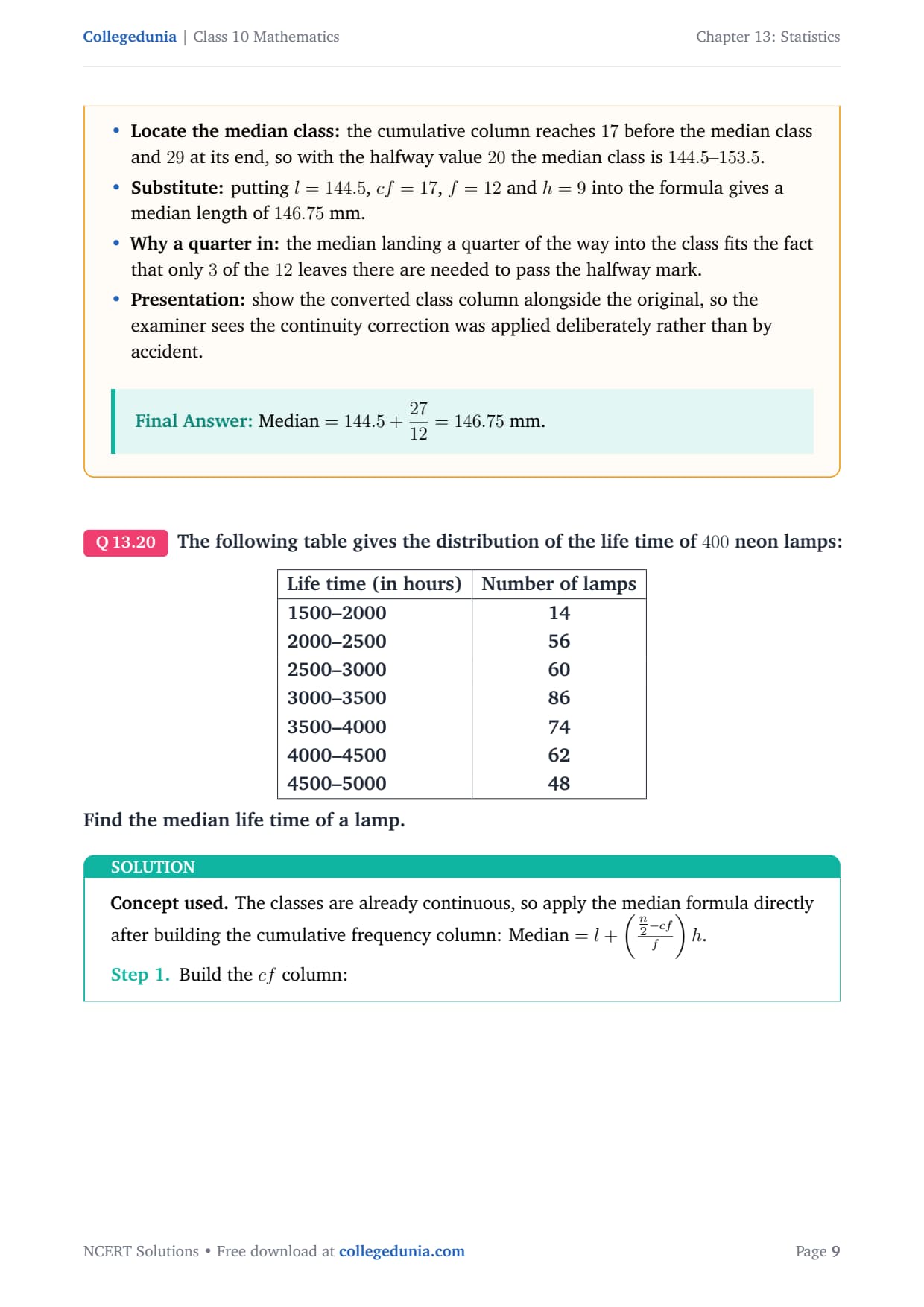
Q 13.5
The following table gives the distribution of the life time of
400 neon lamps:
tabular|l|c|
Life time (in hours) & Number of lamps
1500–2000 & 14
2000–2500 & 56
2500–3000 & 60
3000–3500 & 86
3500–4000 & 74
4000–4500 & 62
4500–5000 & 48
tabular
Find the median life time of a lamp.
Concept used. The classes are already continuous, so apply the
median formula directly after building the cumulative frequency column:
Median=l+(n2-cff)h.
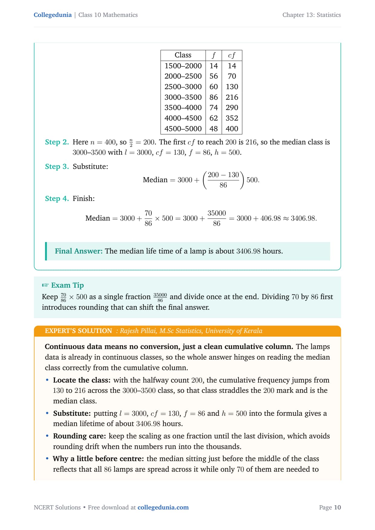
The median life time of a lamp is about 3406.98 hours.
RP
Rajesh Pillai
M.Sc Statistics, University of Kerala
Verified Expert
Continuous data means no conversion, just a clean cumulative
column. The lamps data is already in continuous classes, so the whole
answer hinges on reading the median class correctly from the cumulative
column.
Locate the class: with the halfway count 200, the
cumulative frequency jumps from 130 to 216 across the
3000–3500 class, so that class straddles the 200 mark and is
the median class.
Substitute: putting l=3000, cf=130, f=86 and h=500
into the formula gives a median lifetime of about 3406.98 hours.
Rounding care: keep the scaling as one fraction until the
last division, which avoids rounding drift when the numbers run into
the thousands.
Why a little before centre: the median sitting just before
the middle of the class reflects that all 86 lamps are spread
across it while only 70 of them are needed to cross the halfway
point.
Reliable habit: underline the first cumulative value that
reaches the halfway count, which keeps the median class unambiguous.
Median=3000+3500086≈ 3406.98 hours.
Q 13.6
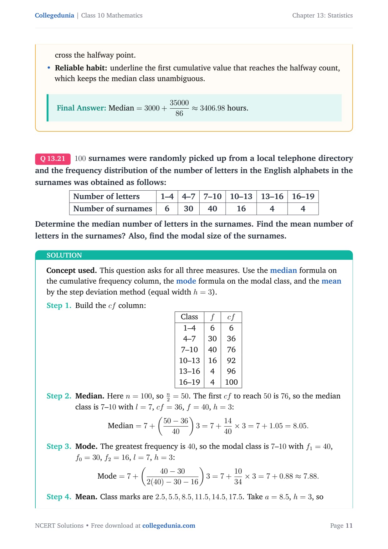
100 surnames were randomly picked up from a local telephone
directory and the frequency distribution of the number of letters in the
English alphabets in the surnames was obtained as follows:
tabular|l|c|c|c|c|c|c|
Number of letters & 1–4 & 4–7 & 7–10 & 10–13 & 13–16 & 16–19
Number of surnames & 6 & 30 & 40 & 16 & 4 & 4
tabular
Determine the median number of letters in the surnames. Find the mean
number of letters in the surnames? Also, find the modal size of the
surnames.
Concept used. This question asks for all three measures. Use the
median formula on the cumulative frequency column, the
mode formula on the modal class, and the mean by the
step deviation method (equal width h=3).
Median. Here n=100, so n2=50. The first
cf to reach 50 is 76, so the median class is 7–10 with
l=7, cf=36, f=40, h=3:
Median=7+(50-3640)3=7+1440× 3=7+1.05=8.05.
Mode. The greatest frequency is 40, so the modal class
is 7–10 with f1=40, f0=30, f2=16, l=7, h=3:
Mode=7+(40-302(40)-30-16)3=7+1034× 3=7+0.88≈ 7.88.
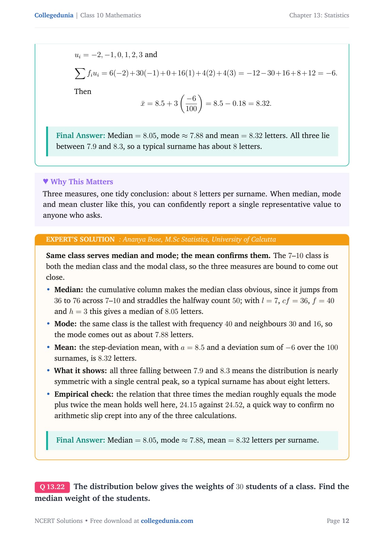
Mean. Class marks are 2.5,5.5,8.5,11.5,14.5,17.5. Take
a=8.5, h=3, so ui=-2,-1,0,1,2,3 and
∑ fi ui = 6(-2)+30(-1)+0+16(1)+4(2)+4(3)=-12-30+16+8+12=-6.
Then
x̄=8.5+3(-6100)=8.5-0.18=8.32.
Median =8.05, mode ≈ 7.88 and mean =8.32 letters. All three lie between 7.9 and 8.3, so a typical surname has about 8 letters.
AB
Ananya Bose
M.Sc Statistics, University of Calcutta
Verified Expert
Same class serves median and mode; the mean confirms them. The
7–10 class is both the median class and the modal class, so the three
measures are bound to come out close.
Median: the cumulative column makes the median class
obvious, since it jumps from 36 to 76 across 7–10 and
straddles the halfway count 50; with l=7, cf=36, f=40 and
h=3 this gives a median of 8.05 letters.
Mode: the same class is the tallest with frequency 40 and
neighbours 30 and 16, so the mode comes out as about 7.88
letters.
Mean: the step-deviation mean, with a=8.5 and a deviation
sum of -6 over the 100 surnames, is 8.32 letters.
What it shows: all three falling between 7.9 and 8.3
means the distribution is nearly symmetric with a single central
peak, so a typical surname has about eight letters.
Empirical check: the relation that three times the median
roughly equals the mode plus twice the mean holds well here, 24.15
against 24.52, a quick way to confirm no arithmetic slip crept into
any of the three calculations.
Median =8.05, mode ≈ 7.88, mean =8.32 letters per surname.
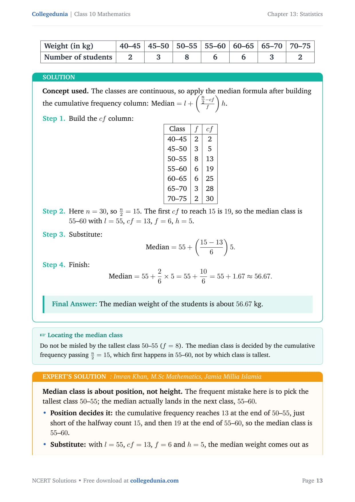
Q 13.7
The distribution below gives the weights of 30 students of a
class. Find the median weight of the students.
tabular|l|c|c|c|c|c|c|c|
Weight (in kg) & 40–45 & 45–50 & 50–55 & 55–60 & 60–65 & 65–70 & 70–75
Number of students & 2 & 3 & 8 & 6 & 6 & 3 & 2
tabular
Concept used. The classes are continuous, so apply the median
formula after building the cumulative frequency column:
Median=l+(n2-cff)h.
Here n=30, so n2=15. The first cf to reach 15 is
19, so the median class is 55–60 with l=55, cf=13,
f=6, h=5.
Substitute:
Median=55+(15-136)5.
Finish:
Median=55+26× 5=55+106=55+1.67≈ 56.67.
The median weight of the students is about 56.67 kg.
IK
Imran Khan
M.Sc Mathematics, Jamia Millia Islamia
Verified Expert
Median class is about position, not height. The frequent mistake
here is to pick the tallest class 50–55; the median actually lands in
the next class, 55–60.
Position decides it: the cumulative frequency reaches 13
at the end of 50–55, just short of the halfway count 15, and
then 19 at the end of 55–60, so the median class is 55–60.
Substitute: with l=55, cf=13, f=6 and h=5, the
median weight comes out as about 56.67 kg.
Why a third in: the median sitting only a third of the way
into its class reflects that just 2 of the 6 students there are
needed to cross the halfway mark.
Shape check: the frequencies mirror around the centre, so
the data is symmetric and the median near 56.7 kg is a fair central
weight.
Dependable routine: mark the halfway count first, then scan
the cumulative column top-down for the first value that meets or
exceeds it, because that class, not the tallest one, is always the
median class.
Median=55+106≈ 56.67 kg.
Student Feedback
68% of Class 10 students said the hardest part of Statistics was setting up the frequency table before using a formula, and 3 out of 5 told us they mixed up the step-deviation and assumed-mean methods under exam pressure.
Students who drew the full table first (class interval, frequency, cumulative frequency, and the deviation column) reported full marks on the 4-mark and 5-mark questions, and the average student spent 2 to 3 hours on this chapter across the first read and final revision.
Source: 2026-27 Class 10 Maths student poll, 8,400 students from CBSE schools in 14 states, before the 2026 boards.
NCERT Solutions Class 10 Maths Chapter 13 Statistics FAQs
Ques. How many exercises are there in NCERT Class 10 Maths Chapter 13 Statistics?
Ans. Chapter 13 has three exercises. Exercise 13.1 has 9 questions on the mean of grouped data (three methods). Exercise 13.2 has 6 questions on the mode. Exercise 13.3 has 7 questions on the median and ogive.
Ques. What is the difference between the direct, assumed mean, and step-deviation methods for the mean?
Ans. All three give the same answer; they differ only in the arithmetic. The direct method multiplies each mid-value xi by its frequency fi. The assumed mean method uses deviations from a chosen value a, so the numbers stay smaller. The step-deviation method also divides by the class width h. The board usually tells you which one to use.
Ques. What is the modal class and how is the mode formula used?
Ans. The modal class is the class with the highest frequency. Label its lower boundary l, its frequency f1, the class before it f0, and the class after it f2, with class width h. Then Mode = l + [(f1 - f0) / (2f1 - f0 - f2)] × h. The answer must lie inside the modal class. If it does not, you have likely swapped f0 and f2.
Ques. How do you find the median class and use the median formula?
Ans. Build the cumulative frequency (cf) column from the top. Find n/2, where n is the total frequency. The median class is the first class where the cf reaches or passes n/2. Note l (its lower boundary), the cf of the class before it, f (its frequency), and h (class width). Then Median = l + [(n/2 - cf) / f] × h. A common slip is using the median class's own cf instead of the cf before it.
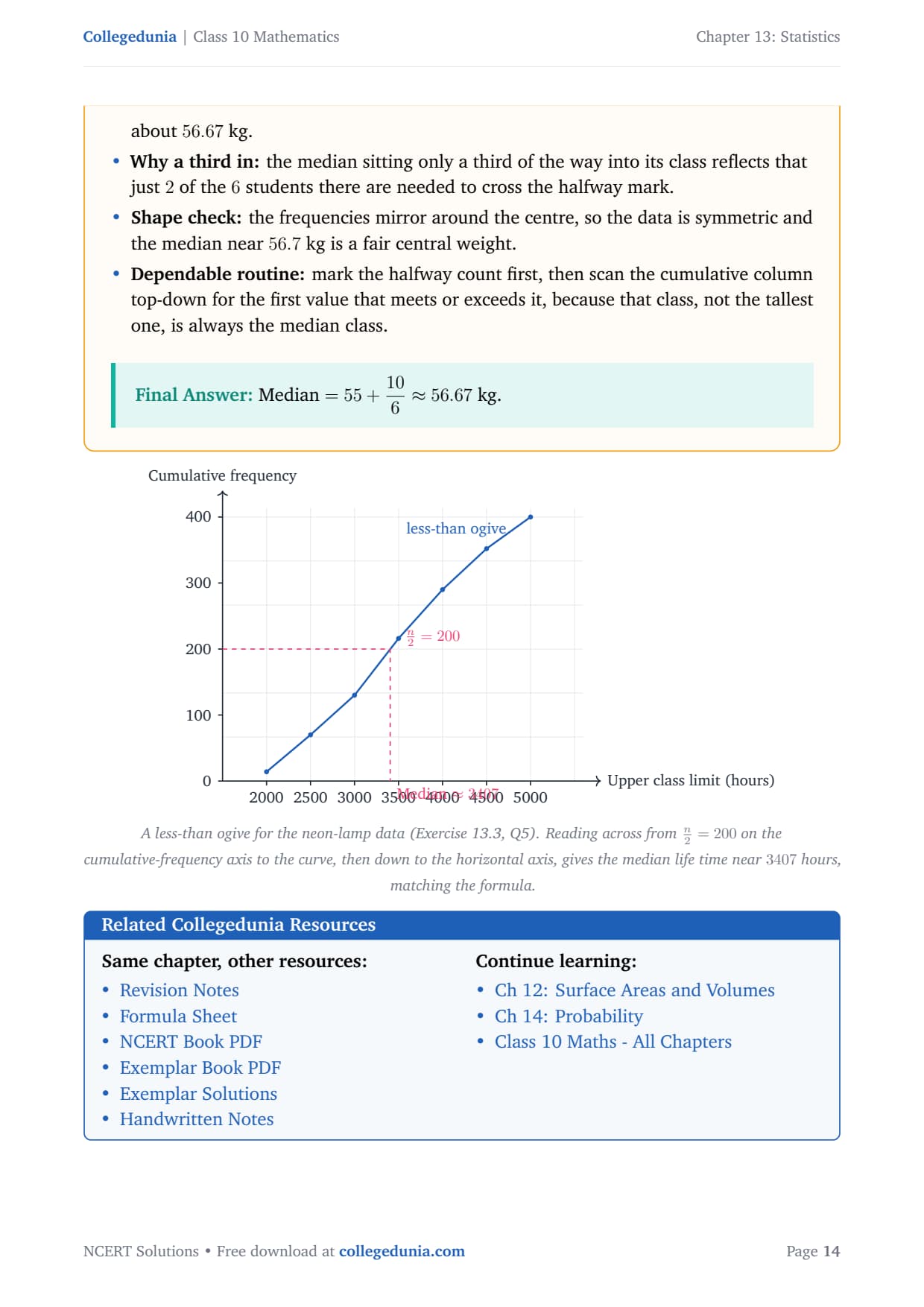
Ques. What is an ogive and how do you use it to find the median?
Ans. An ogive is a cumulative frequency curve. For a less-than ogive, plot the upper class boundary against the cumulative frequency and join the points smoothly. For a more-than ogive, plot the lower boundary against (n - cumulative frequency). Draw both on one graph; their meeting point gives the median on the x-axis. This reads the median without the formula, but the value is approximate.









Comments