Maths Strategist, Olympiad Coach | Updated 3+ months ago
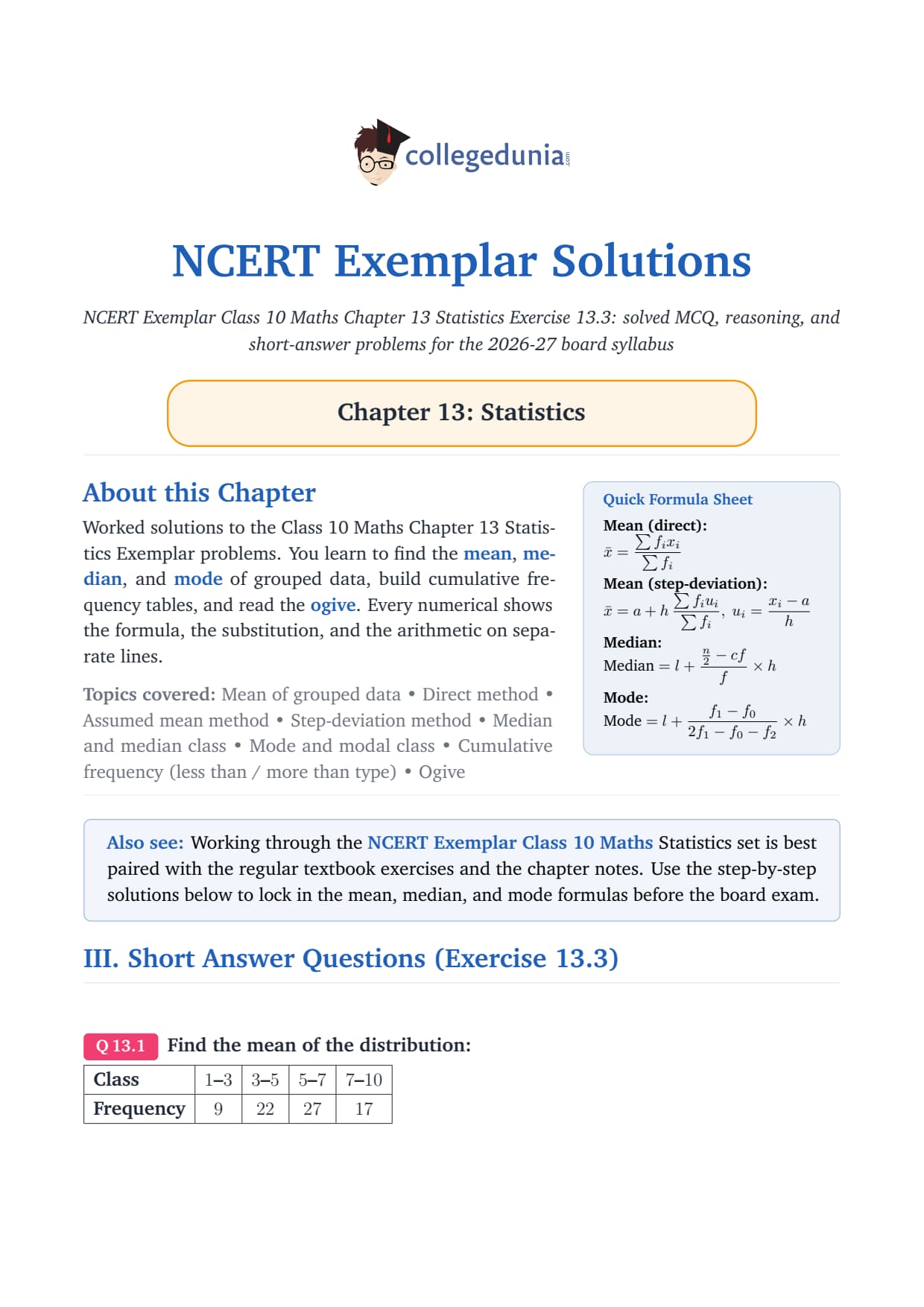
Class 10 Maths Chapter 13 Statistics Exercise 13.3 is the Short Answer section of the NCERT Exemplar. It has 18 questions covering mean by three methods, cumulative frequency tables, ogive construction, median, and mode for grouped data, according to the 2026-27 CBSE syllabus.
18 Short Answer Questions with full step-by-step solutions, expert analysis, and common-mistake warnings for each problem in Exercise 13.3.
Key concepts tested: direct method, assumed mean method, and step-deviation method for mean; less than and more than type cumulative frequency; median and mode for grouped data.
CBSE Weightage: Statistics carries 5 to 6 marks in the Class 10 board paper, usually one 3-mark and one 5-mark question picked from this chapter.
Each NCERT Exemplar solution for Class 10 Maths Chapter 13 Exercise 13.3 on this page is curated by subject experts, mapped to the 2026-27 NCERT Exemplar book, and checked against the last five years of CBSE board papers for this chapter.
Solved by Collegedunia
All 18 questions of Exercise 13.3 are solved below with Concept, Step-by-step working, and an Expert's insight for each.
Exercise 13.3 is the Short Answer section of the NCERT Exemplar for Chapter 13 Statistics. It has 18 questions numbered Q1 to Q18 (internally Q16 to Q33 in the full Exemplar book). The questions span mean by three methods, cumulative frequency tables, and median/mode for grouped data.
Question Range
Topic Focus
Key Idea
Q1
Mean with unequal class widths
Direct method; class mark of the wider last class
Q2
Mean of test scores
Direct method; assumed-mean cross-check
Q3
Mean with inclusive classes
No continuity correction needed for mean
Q4
Mean pages per day
Step-deviation method; equal class widths
Q5
Mean income with inclusive money brackets
Class marks end in 0.5; carry the half-unit
Q6
Mean seats in aircraft flights
Step-deviation; small negative correction
Q7
Mean weight of wrestlers
Step-deviation; correction decodes to real kg
Q8
Mean mileage + claim verdict
Compute mean, then compare with claim
Q9
Construct less than cumulative frequency
Running total; final entry = total
Q10
Recover frequency from below cumulative
Successive differences; first class is special
Q11
Recover frequency from more than cumulative
Top-down differencing
Q12
Find unknown entries in cumulative table
Running total rule; use stated total as check
Q13
Build both cumulative distributions
Less than (add) and more than (subtract from total)
Q14
Frequency from below cumulative (wide classes)
Differences; modal class hidden until differenced
Q15
Median income of 600 families
Median class from cumulative column
Q16
Median bowling speed
Fractional n2 is expected with odd n
Q17
Modal monthly income
Mode formula; denominator shortcut
Q18
Modal weight of coffee packets
h = 1 (narrow classes); mode barely inside modal class
The difficulty ranges from moderate (Q1-Q9) to higher-order (Q10-Q14 on cumulative tables). Median and mode questions (Q15-Q18) are the ones CBSE picks most often for the 5-mark board question.
Key Formulas for Exercise 13.3
Every question in Exercise 13.3 uses one or more of these formulas. Memorise the triggering condition for each method so you pick the right one on the board paper.
Formula
When to Use
Key Symbol
Used in
Mean (Direct Method) x = ∑ fi xi∑ fi
Any class width (especially unequal widths)
xi = class mark
Q1, Q2, Q3, Q5
Mean (Step-Deviation) x = a + h ∑ fi ui∑ fi
where ui = xi − ah
Equal class widths (large numbers)
a = assumed mean; h = width
Q4, Q6, Q7, Q8
Median l + n2 − cff × h
Grouped data; after locating median class
cf = preceding cumulative frequency
Q15, Q16
Mode l + f1 − f02f1 − f0 − f2 × h
Grouped data; after identifying modal class
f1 = modal class freq
Q17, Q18
Less than cumulative
Running total from top class
Upper boundary on X-axis for ogive
Q9, Q10, Q13, Q14
More than cumulative
Subtract from grand total downward
Lower boundary on X-axis for ogive
Q11, Q13
Use the step-deviation method whenever class widths are equal and numbers are large, it turns messy products into small integers. Switch to the direct method when widths differ (like Q1) or the numbers are already small.
Common Mistakes to Avoid
Exercise 13.3 problems are built so each common error leads to a specific wrong answer the examiner has already seen. Knowing these saves 5 to 6 marks on the CBSE board paper.
Question
Common Mistake
The Fix
Q1
Using class mark 9 for the last class 7–10
Correct mark:7+102 = 8.5. The class is wider, so average both limits.
Q3
Applying a continuity correction to the class marks before computing mean
No correction needed for the mean. Continuity correction shifts boundaries but leaves mid-points unchanged.
Q5
Rounding class mark of 1–200 to 100 instead of 100.5
Always average the stated limits exactly: 1+2002 = 100.5.
Q6
Adding instead of subtracting when ∑ fi ui is negative
A negative sum means the mean is below a. The correction is -0.08, giving 109.92.
Q10
Treating the first class as a difference from zero
First class frequency = first cumulative entry directly. Only later classes are differences.
Q15
Choosing 0–1000 as the median class because it has the largest frequency
Median class is determined by cumulative frequency, not by the largest frequency. Here n2=300 falls inside 1000–2000.
Q18
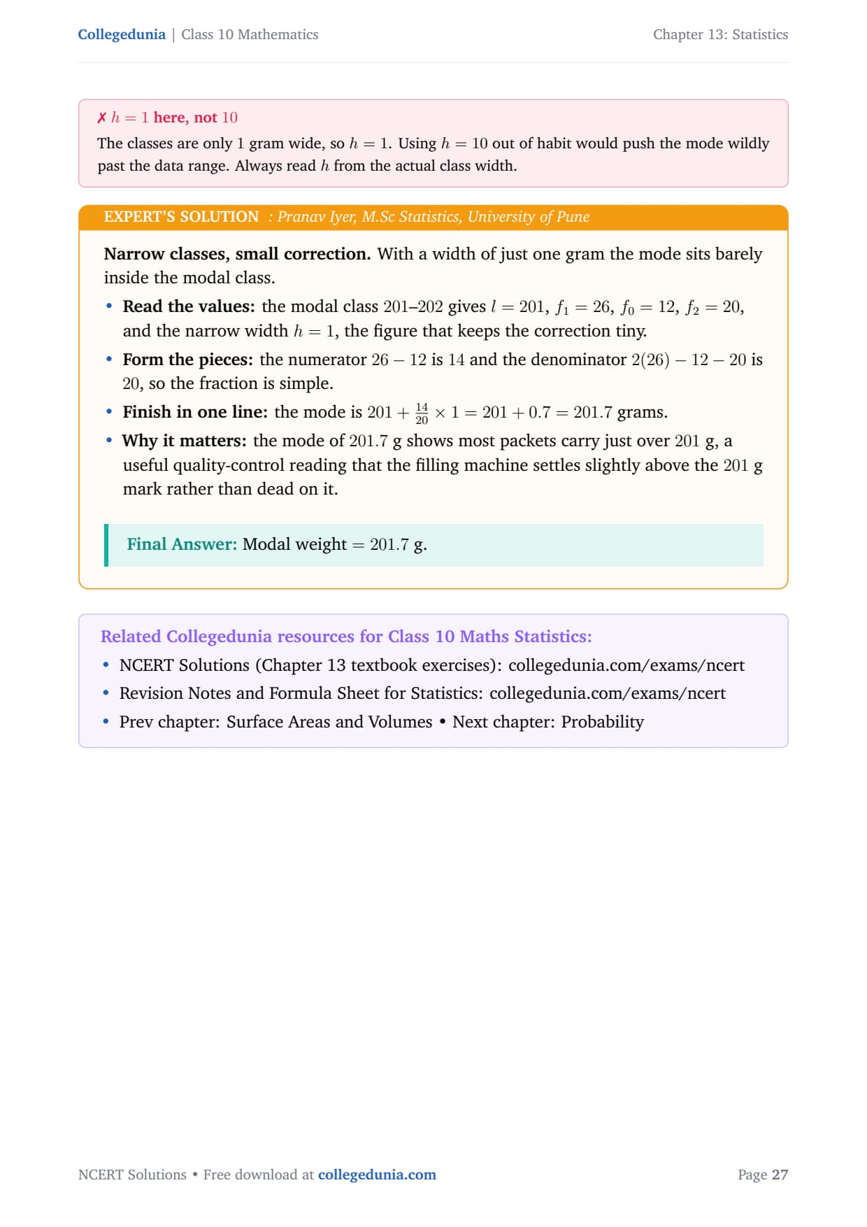
Using h = 10 out of habit
The classes are 1 gram wide, so h = 1. Always read h from the actual class width.
Question Types and Difficulty
All Exercise 13.3 Questions with Step-by-Step Solutions
III. Short Answer Questions (Exercise 13.3)
Q 13.1
Find the mean of the distribution: [2pt]
tabular|l|c|c|c|c|
Class & 1–3 & 3–5 & 5–7 & 7–10
Frequency & 9 & 22 & 27 & 17
tabular
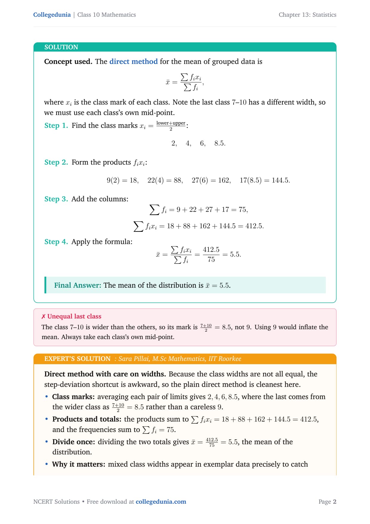
Concept used. The direct method for the mean of
grouped data is
x̄=∑ fi xi∑ fi,
where xi is the class mark of each class. Note the last class
7–10 has a different width, so we must use each class's own
mid-point.
Find the class marks xi=lower+upper2:
2, 4, 6, 8.5.
Form the products fi xi:
9(2)=18, 22(4)=88, 27(6)=162, 17(8.5)=144.5.
Add the columns:
∑ fi = 9+22+27+17 = 75, ∑ fi xi = 18+88+162+144.5 = 412.5.
Apply the formula:
x̄=∑ fi xi∑ fi
=412.575
=5.5.
The mean of the distribution is x̄=5.5.
SP
Sara Pillai
M.Sc Mathematics, IIT Roorkee
Verified Expert
Direct method with care on widths. Because the class widths are
not all equal, the step-deviation shortcut is awkward, so the plain
direct method is cleanest here.
Class marks: averaging each pair of limits gives
2,4,6,8.5, where the last comes from the wider class as
7+102=8.5 rather than a careless 9.
Products and totals: the products sum to
∑ fi xi = 18+88+162+144.5 = 412.5, and the frequencies
sum to ∑ fi = 75.
Divide once: dividing the two totals gives
x̄=412.575=5.5, the mean of the distribution.
Why it matters: mixed class widths appear in exemplar
data precisely to catch students who memorise one class mark and
reuse it, so recomputing xi for every class is the safe habit.
x̄=5.5.
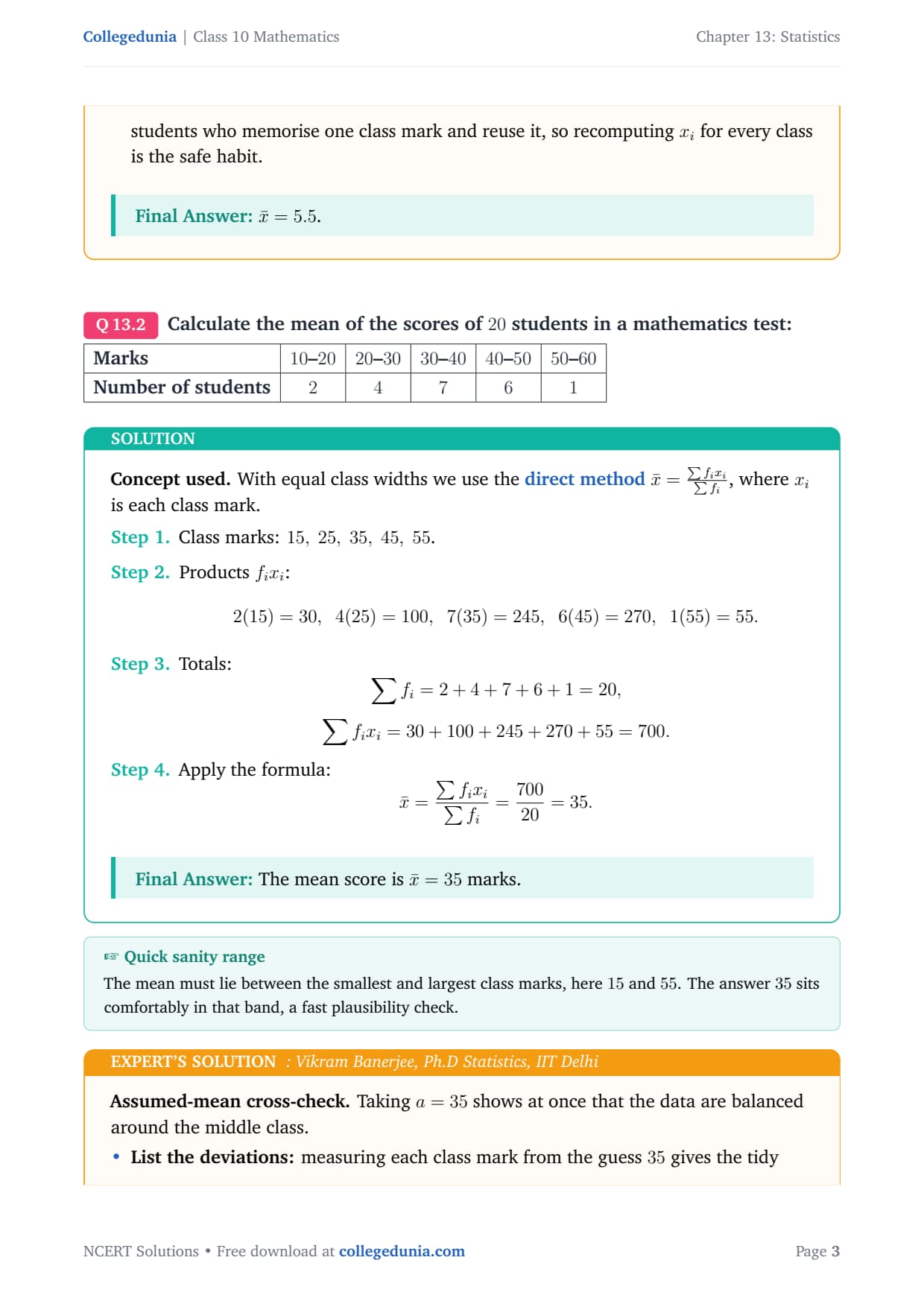
Q 13.2
Calculate the mean of the scores of 20 students in a mathematics test: [2pt]
tabular|l|c|c|c|c|c|
Marks & 10–20 & 20–30 & 30–40 & 40–50 & 50–60
Number of students & 2 & 4 & 7 & 6 & 1
tabular
Concept used. With equal class widths we use the direct
methodx̄=∑ fi xi∑ fi, where xi is each
class mark.
Class marks: 15, 25, 35, 45, 55.
Products fi xi:
2(15)=30, 4(25)=100, 7(35)=245, 6(45)=270, 1(55)=55.
Totals:
∑ fi = 2+4+7+6+1 = 20, ∑ fi xi = 30+100+245+270+55 = 700.
Apply the formula:
x̄=∑ fi xi∑ fi
=70020
=35.
The mean score is x̄=35 marks.
VB
Vikram Banerjee
Ph.D Statistics, IIT Delhi
Verified Expert
Assumed-mean cross-check. Taking a=35 shows at once that the
data are balanced around the middle class.
List the deviations: measuring each class mark from the
guess 35 gives the tidy values -20,-10,0,10,20.
Sum them weighted: the weighted total
∑ fi di = 2(-20)+4(-10)+0+6(10)+1(20) collapses to exactly
zero once the negatives and positives cancel.
Recover the mean: feeding that zero into
x̄=a+∑ fi di∑ fi=35+020 leaves
35, in full agreement with the direct method.
Why it matters: a zero deviation sum is a signal that
the data are symmetric about the guess, so the assumed mean is
already the true mean, which is the fastest possible finish when
it happens.
x̄=35 marks.
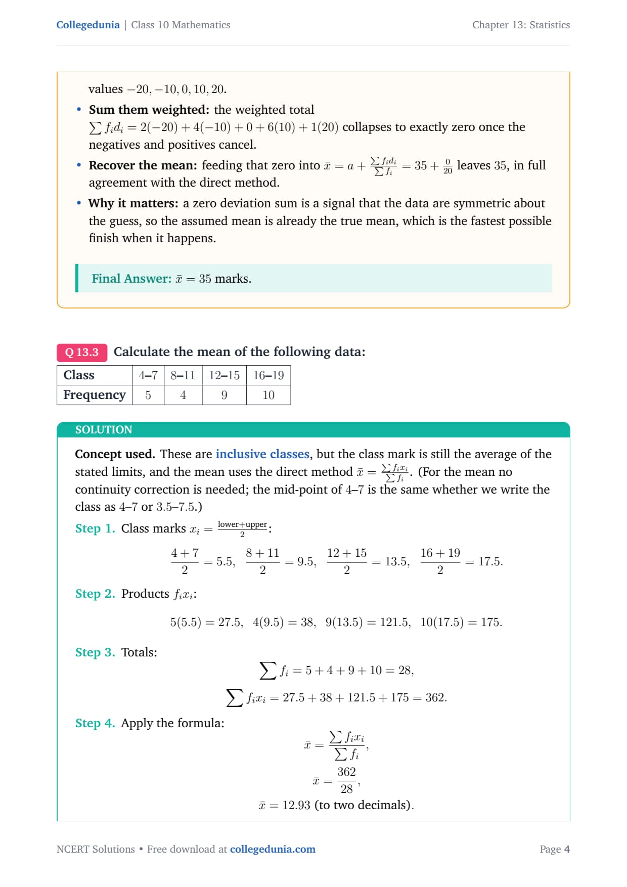
Q 13.3
Calculate the mean of the following data: [2pt]
tabular|l|c|c|c|c|
Class & 4–7 & 8–11 & 12–15 & 16–19
Frequency & 5 & 4 & 9 & 10
tabular
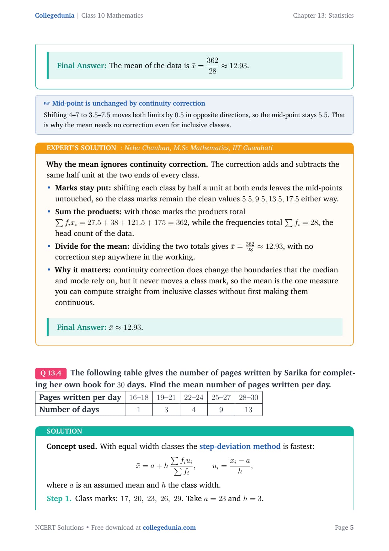
Concept used. These are inclusive classes, but the
class mark is still the average of the stated limits, and the mean uses
the direct method x̄=∑ fi xi∑ fi. (For the mean
no continuity correction is needed; the mid-point of 4–7 is the same
whether we write the class as 4–7 or 3.5–7.5.)
Class marks xi=lower+upper2:
4+72=5.5, 8+112=9.5,
12+152=13.5, 16+192=17.5.
Products fi xi:
5(5.5)=27.5, 4(9.5)=38, 9(13.5)=121.5, 10(17.5)=175.
Totals:
∑ fi = 5+4+9+10 = 28, ∑ fi xi = 27.5+38+121.5+175 = 362.
Apply the formula:
x̄=∑ fi xi∑ fi, x̄=36228, x̄=12.93 (to two decimals).
The mean of the data is x̄=36228≈ 12.93.
NC
Neha Chauhan
M.Sc Mathematics, IIT Guwahati
Verified Expert
Why the mean ignores continuity correction. The correction adds
and subtracts the same half unit at the two ends of every class.
Marks stay put: shifting each class by half a unit at
both ends leaves the mid-points untouched, so the class marks
remain the clean values 5.5,9.5,13.5,17.5 either way.
Sum the products: with those marks the products total
∑ fi xi = 27.5+38+121.5+175 = 362, while the frequencies
total ∑ fi = 28, the head count of the data.
Divide for the mean: dividing the two totals gives
x̄=36228≈ 12.93, with no correction step
anywhere in the working.
Why it matters: continuity correction does change the
boundaries that the median and mode rely on, but it never moves a
class mark, so the mean is the one measure you can compute
straight from inclusive classes without first making them
continuous.
x̄≈ 12.93.
Q 13.4
The following table gives the number of pages written by Sarika for completing her own book for 30 days. Find the mean number of pages written per day. [2pt]
tabular|l|c|c|c|c|c|
Pages written per day & 16–18 & 19–21 & 22–24 & 25–27 & 28–30
Number of days & 1 & 3 & 4 & 9 & 13
tabular
Concept used. With equal-width classes the step-deviation
method is fastest:
x̄=a+h∑ fi ui∑ fi, ui=xi-ah,
where a is an assumed mean and h the class width.
Class marks: 17, 20, 23, 26, 29. Take a=23 and
h=3.
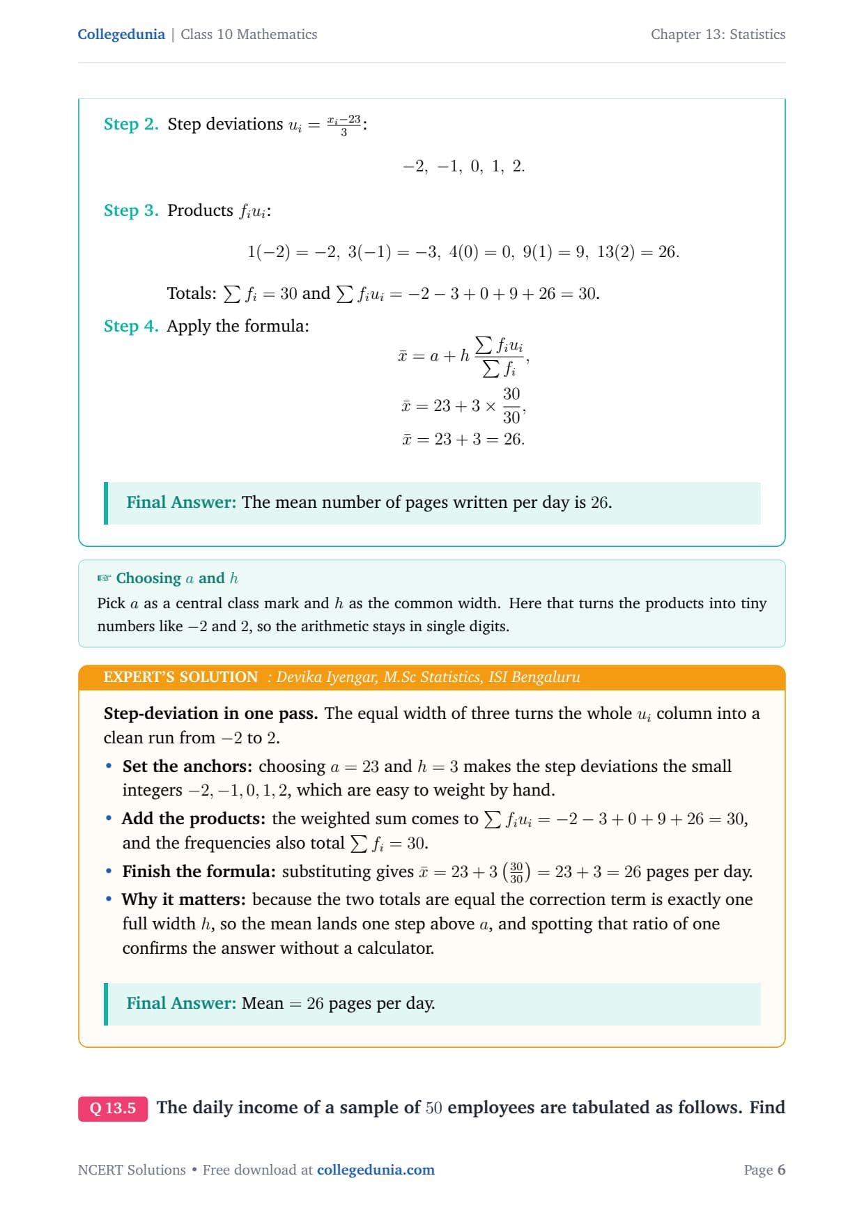
Step deviations ui=xi-233:
-2, -1, 0, 1, 2.
Products fi ui:
1(-2)=-2, 3(-1)=-3, 4(0)=0, 9(1)=9, 13(2)=26.
Totals: ∑ fi = 30 and
∑ fi ui = -2-3+0+9+26 = 30.
Apply the formula:
x̄=a+h∑ fi ui∑ fi, x̄=23+3×3030, x̄=23+3=26.
The mean number of pages written per day is 26.
DI
Devika Iyengar
M.Sc Statistics, ISI Bengaluru
Verified Expert
Step-deviation in one pass. The equal width of three turns the
whole ui column into a clean run from -2 to 2.
Set the anchors: choosing a=23 and h=3 makes the
step deviations the small integers -2,-1,0,1,2, which are easy
to weight by hand.
Add the products: the weighted sum comes to
∑ fi ui = -2-3+0+9+26 = 30, and the frequencies also total
∑ fi = 30.
Finish the formula: substituting gives
x̄=23+3(3030)=23+3=26 pages per day.
Why it matters: because the two totals are equal the
correction term is exactly one full width h, so the mean lands
one step above a, and spotting that ratio of one confirms the
answer without a calculator.
Mean =26 pages per day.
Q 13.5
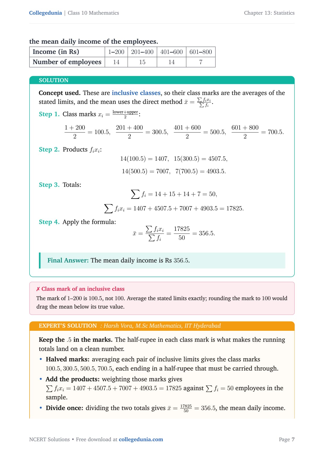
The daily income of a sample of 50 employees are tabulated as follows. Find the mean daily income of the employees. [2pt]
tabular|l|c|c|c|c|
Income (in Rs) & 1–200 & 201–400 & 401–600 & 601–800
Number of employees & 14 & 15 & 14 & 7
tabular
Concept used. These are inclusive classes, so their
class marks are the averages of the stated limits, and the mean uses the
direct method x̄=∑ fi xi∑ fi.
Class marks xi=lower+upper2:
1+2002=100.5, 201+4002=300.5,
401+6002=500.5, 601+8002=700.5.
Products fi xi:
14(100.5)=1407, 15(300.5)=4507.5, 14(500.5)=7007, 7(700.5)=4903.5.
Totals:
∑ fi = 14+15+14+7 = 50, ∑ fi xi = 1407+4507.5+7007+4903.5 = 17825.
Apply the formula:
x̄=∑ fi xi∑ fi
=1782550
=356.5.
The mean daily income is Rs 356.5.
HV
Harsh Vora
M.Sc Mathematics, IIT Hyderabad
Verified Expert
Keep the .5 in the marks. The half-rupee in each class mark is
what makes the running totals land on a clean number.
Halved marks: averaging each pair of inclusive limits
gives the class marks 100.5,300.5,500.5,700.5, each ending in a
half-rupee that must be carried through.
Add the products: weighting those marks gives
∑ fi xi = 1407+4507.5+7007+4903.5 = 17825 against
∑ fi = 50 employees in the sample.
Divide once: dividing the two totals gives
x̄=1782550=356.5, the mean daily income.
Why it matters: inclusive money brackets like 1–200
are common in real survey data, and carrying the half-rupee
through the whole table prevents a systematic downward bias in the
reported average income.
Mean daily income = Rs 356.5.
Q 13.6
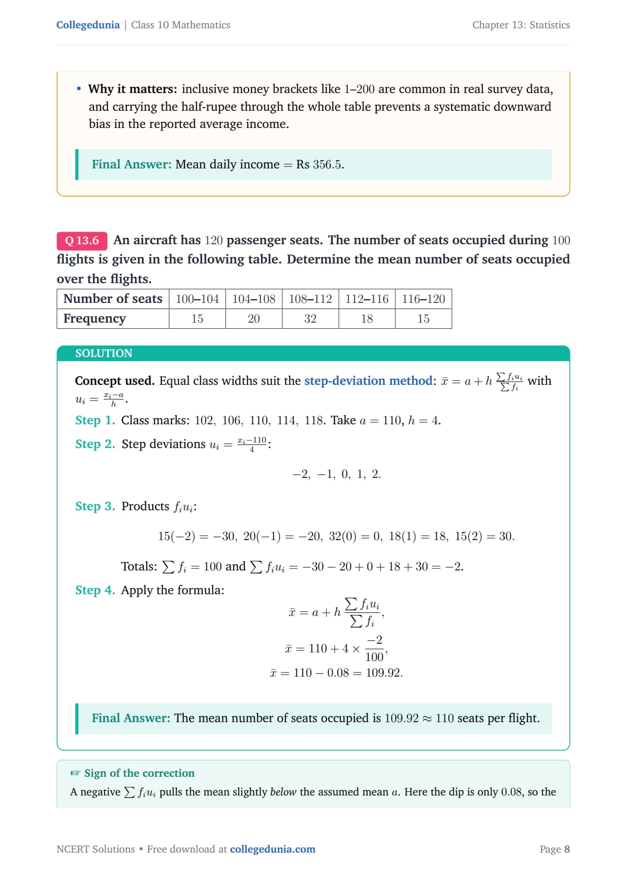
An aircraft has 120 passenger seats. The number of seats occupied during 100 flights is given in the following table. Determine the mean number of seats occupied over the flights. [2pt]
tabular|l|c|c|c|c|c|
Number of seats & 100–104 & 104–108 & 108–112 & 112–116 & 116–120
Frequency & 15 & 20 & 32 & 18 & 15
tabular
Concept used. Equal class widths suit the step-deviation
method: x̄=a+h∑ fi ui∑ fi with
ui=xi-ah.
Class marks: 102, 106, 110, 114, 118. Take a=110, h=4.
Step deviations ui=xi-1104:
-2, -1, 0, 1, 2.
Products fi ui:
15(-2)=-30, 20(-1)=-20, 32(0)=0, 18(1)=18, 15(2)=30.
Totals: ∑ fi = 100 and
∑ fi ui = -30-20+0+18+30 = -2.
Apply the formula:
x̄=a+h∑ fi ui∑ fi, x̄=110+4×-2100, x̄=110-0.08=109.92.
The mean number of seats occupied is 109.92≈ 110 seats per flight.
LP
Lakshmi Pillai
Ph.D Statistics, IISc Bangalore
Verified Expert
Small correction, large a. The assumed mean does the heavy
lifting while the step column only nudges it a little.
Set the anchors: taking a=110 and h=4 gives the
usual step deviations -2,-1,0,1,2, centred on the busiest band.
Add the products: the weighted total is only
∑ fi ui = -2 against a head count of ∑ fi = 100, so
the correction will be small.
Finish the formula: substituting gives
x̄=110+4(-2100)=110-0.08=109.92 seats.
Why it matters: when data are nearly symmetric about the
central class the step sum is tiny and the mean settles very close
to a, which is a handy estimate-first check before you trust the
final decimal.
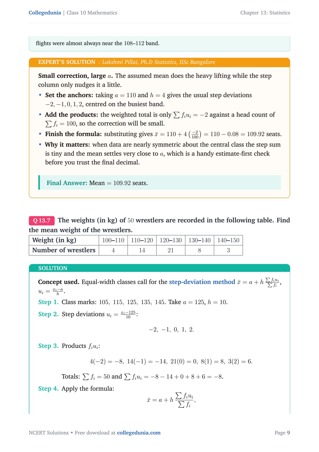
Mean =109.92 seats.
Q 13.7
The weights (in kg) of 50 wrestlers are recorded in the following table. Find the mean weight of the wrestlers. [2pt]
tabular|l|c|c|c|c|c|
Weight (in kg) & 100–110 & 110–120 & 120–130 & 130–140 & 140–150
Number of wrestlers & 4 & 14 & 21 & 8 & 3
tabular
Concept used. Equal-width classes call for the
step-deviation methodx̄=a+h∑ fi ui∑ fi, ui=xi-ah.
Class marks: 105, 115, 125, 135, 145. Take a=125, h=10.
Step deviations ui=xi-12510:
-2, -1, 0, 1, 2.
Products fi ui:
4(-2)=-8, 14(-1)=-14, 21(0)=0, 8(1)=8, 3(2)=6.
Totals: ∑ fi = 50 and
∑ fi ui = -8-14+0+8+6 = -8.
Apply the formula:
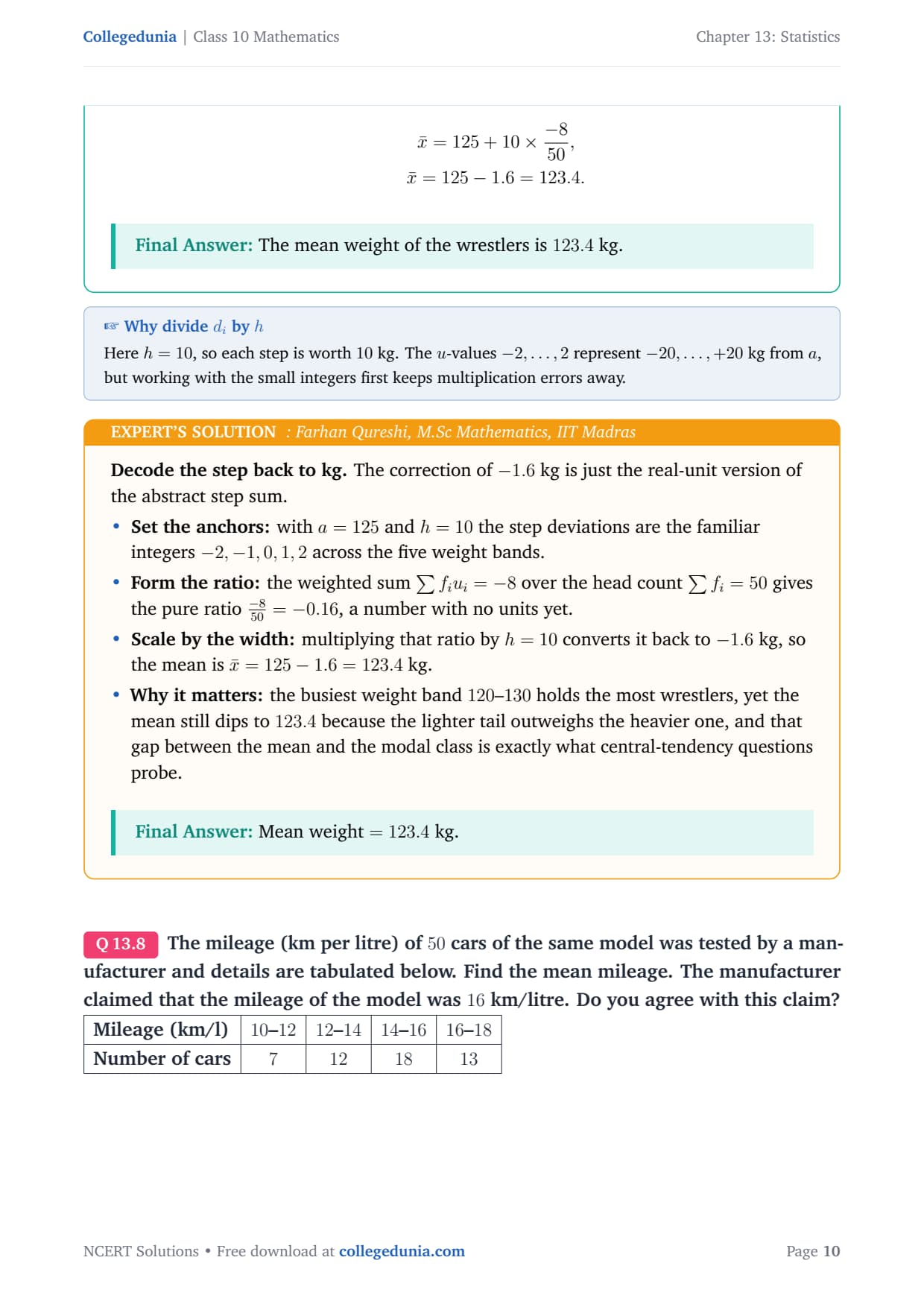
x̄=a+h∑ fi ui∑ fi, x̄=125+10×-850, x̄=125-1.6=123.4.
The mean weight of the wrestlers is 123.4 kg.
FQ
Farhan Qureshi
M.Sc Mathematics, IIT Madras
Verified Expert
Decode the step back to kg. The correction of -1.6 kg is just
the real-unit version of the abstract step sum.
Set the anchors: with a=125 and h=10 the step
deviations are the familiar integers -2,-1,0,1,2 across the five
weight bands.
Form the ratio: the weighted sum ∑ fi ui = -8 over
the head count ∑ fi = 50 gives the pure ratio
-850=-0.16, a number with no units yet.
Scale by the width: multiplying that ratio by h=10
converts it back to -1.6 kg, so the mean is
x̄=125-1.6=123.4 kg.
Why it matters: the busiest weight band 120–130
holds the most wrestlers, yet the mean still dips to 123.4
because the lighter tail outweighs the heavier one, and that gap
between the mean and the modal class is exactly what
central-tendency questions probe.
Mean weight =123.4 kg.
Q 13.8
The mileage (km per litre) of 50 cars of the same model was tested by a manufacturer and details are tabulated below. Find the mean mileage. The manufacturer claimed that the mileage of the model was 16 km/litre. Do you agree with this claim? [2pt]
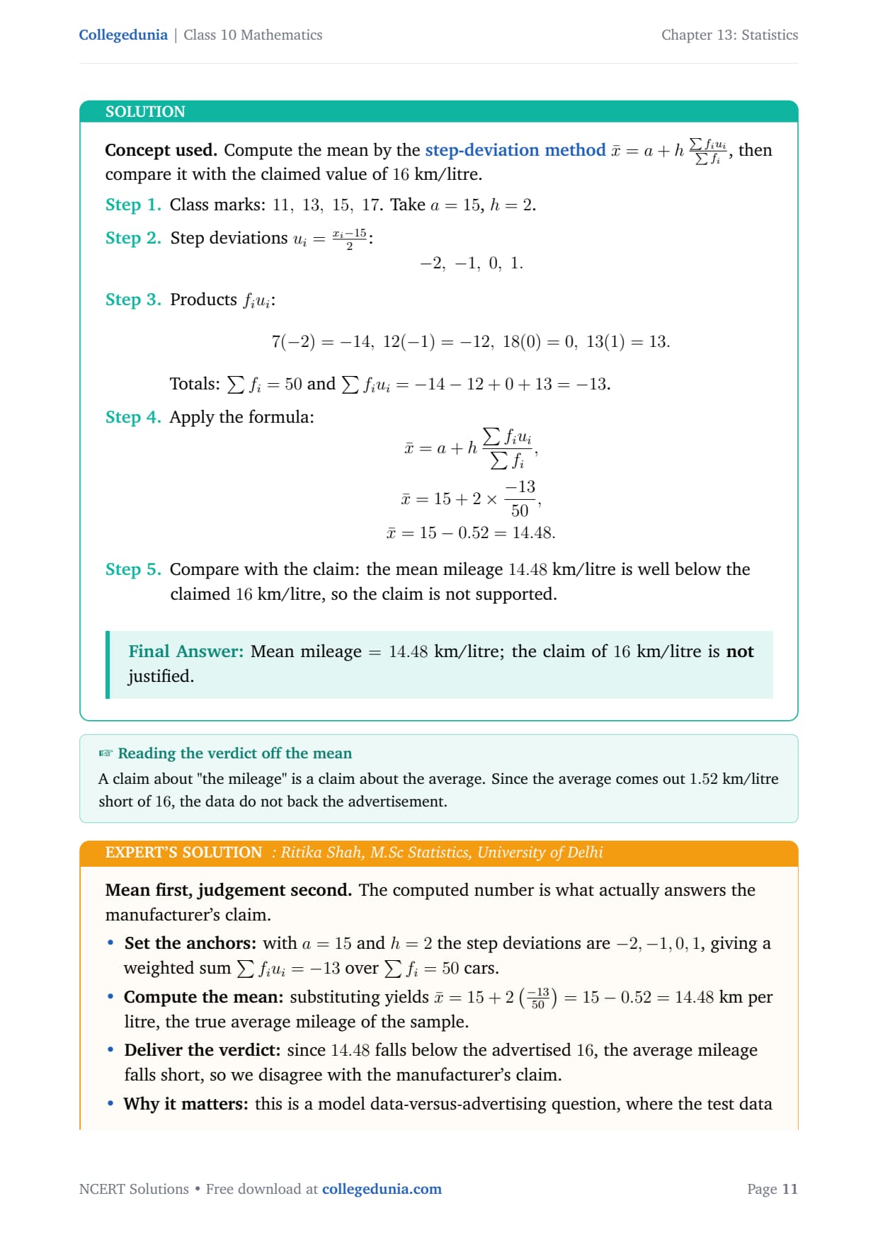
tabular|l|c|c|c|c|
Concept used. Compute the mean by the step-deviation
methodx̄=a+h∑ fi ui∑ fi, then compare it
with the claimed value of 16 km/litre.
Class marks: 11, 13, 15, 17. Take a=15, h=2.
Step deviations ui=xi-152:
-2, -1, 0, 1.
Products fi ui:
7(-2)=-14, 12(-1)=-12, 18(0)=0, 13(1)=13.
Totals: ∑ fi = 50 and
∑ fi ui = -14-12+0+13 = -13.
Apply the formula:
x̄=a+h∑ fi ui∑ fi, x̄=15+2×-1350, x̄=15-0.52=14.48.
Compare with the claim: the mean mileage 14.48 km/litre is
well below the claimed 16 km/litre, so the claim is not
supported.
Mean mileage =14.48 km/litre; the claim of 16 km/litre is not justified.
RS
Ritika Shah
M.Sc Statistics, University of Delhi
Verified Expert
Mean first, judgement second. The computed number is what
actually answers the manufacturer's claim.
Set the anchors: with a=15 and h=2 the step
deviations are -2,-1,0,1, giving a weighted sum
∑ fi ui=-13 over ∑ fi=50 cars.
Compute the mean: substituting yields
x̄=15+2(-1350)=15-0.52=14.48 km per
litre, the true average mileage of the sample.
Deliver the verdict: since 14.48 falls below the
advertised 16, the average mileage falls short, so we disagree
with the manufacturer's claim.
Why it matters: this is a model data-versus-advertising
question, where the test data give a defensible average and any
marketing figure above it must be challenged, so always anchor the
verdict to the computed mean rather than the single best class.
x̄=14.48 km/litre; the 16 km/litre claim is not agreed.
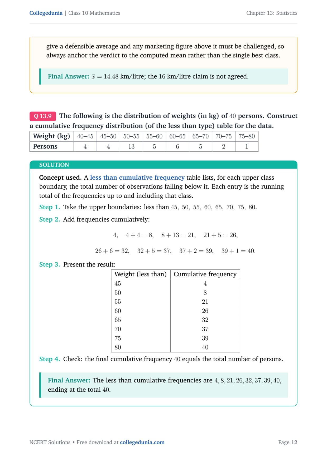
Q 13.9
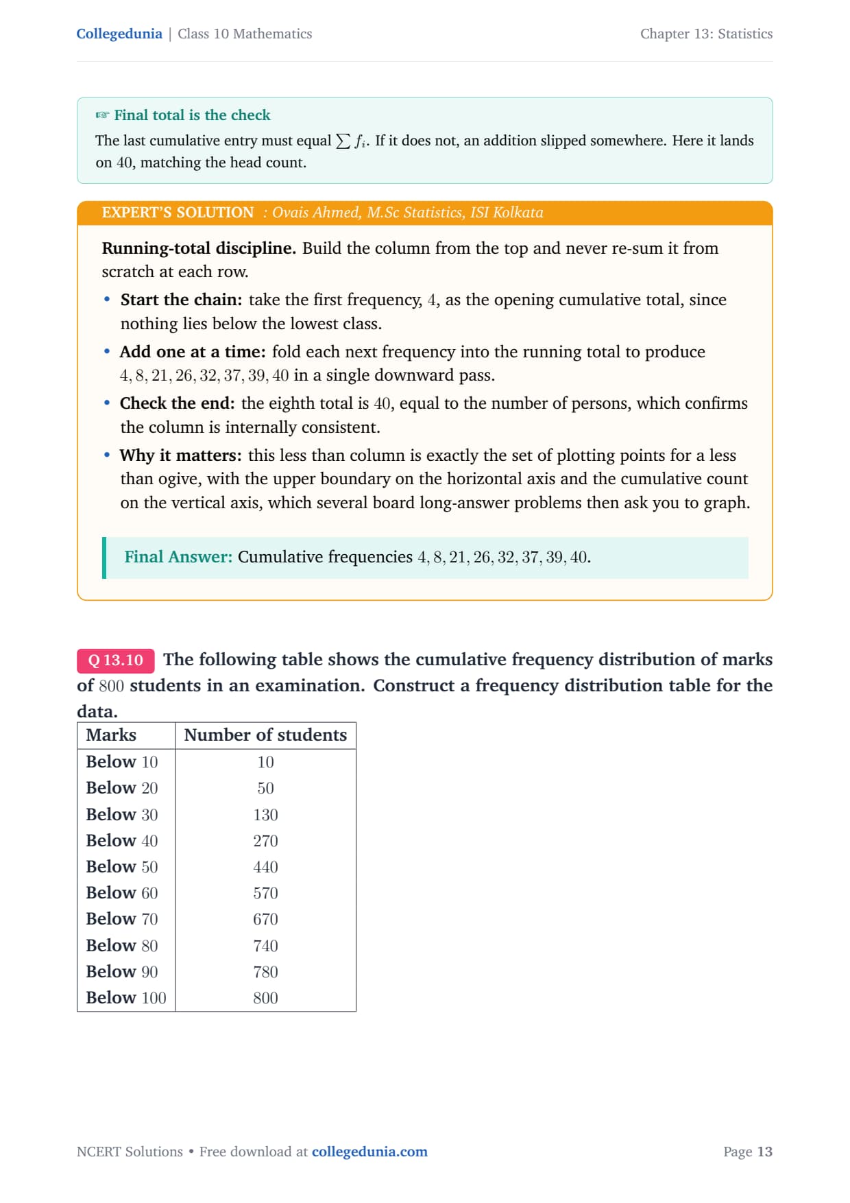
The following is the distribution of weights (in kg) of 40 persons. Construct a cumulative frequency distribution (of the less than type) table for the data. [2pt]
tabular|l|c|c|c|c|c|c|c|c|
Concept used. A less than cumulative frequency table
lists, for each upper class boundary, the total number of observations
falling below it. Each entry is the running total of the frequencies up
to and including that class.
Take the upper boundaries: less than 45, 50, 55, 60, 65,
70, 75, 80.
Check: the final cumulative frequency 40 equals the total
number of persons.
The less than cumulative frequencies are 4,8,21,26,32,37,39,40, ending at the total 40.
OA
Ovais Ahmed
M.Sc Statistics, ISI Kolkata
Verified Expert
Running-total discipline. Build the column from the top and
never re-sum it from scratch at each row.
Start the chain: take the first frequency, 4, as the
opening cumulative total, since nothing lies below the lowest
class.
Add one at a time: fold each next frequency into the
running total to produce 4,8,21,26,32,37,39,40 in a single
downward pass.
Check the end: the eighth total is 40, equal to the
number of persons, which confirms the column is internally
consistent.
Why it matters: this less than column is exactly the set
of plotting points for a less than ogive, with the upper boundary
on the horizontal axis and the cumulative count on the vertical
axis, which several board long-answer problems then ask you to
graph.
Cumulative frequencies 4,8,21,26,32,37,39,40.
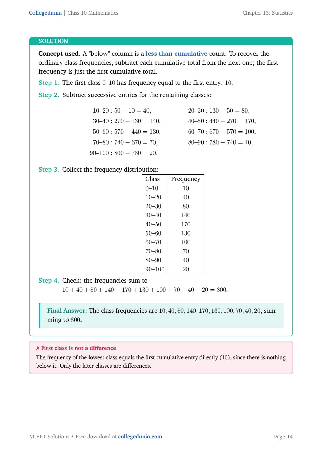
Q 13.10
The following table shows the cumulative frequency distribution of marks of 800 students in an examination. Construct a frequency distribution table for the data. [2pt]
tabular|l|c|
Concept used. A "below" column is a less than
cumulative count. To recover the ordinary class frequencies, subtract
each cumulative total from the next one; the first frequency is just the
first cumulative total.
The first class 0–10 has frequency equal to the first entry:
10.
Check: the frequencies sum to
10+40+80+140+170+130+100+70+40+20 = 800.
The class frequencies are 10,40,80,140,170,130,100,70,40,20, summing to 800.
BR
Bhavna Reddy
M.Sc Mathematics, IIT Bombay
Verified Expert
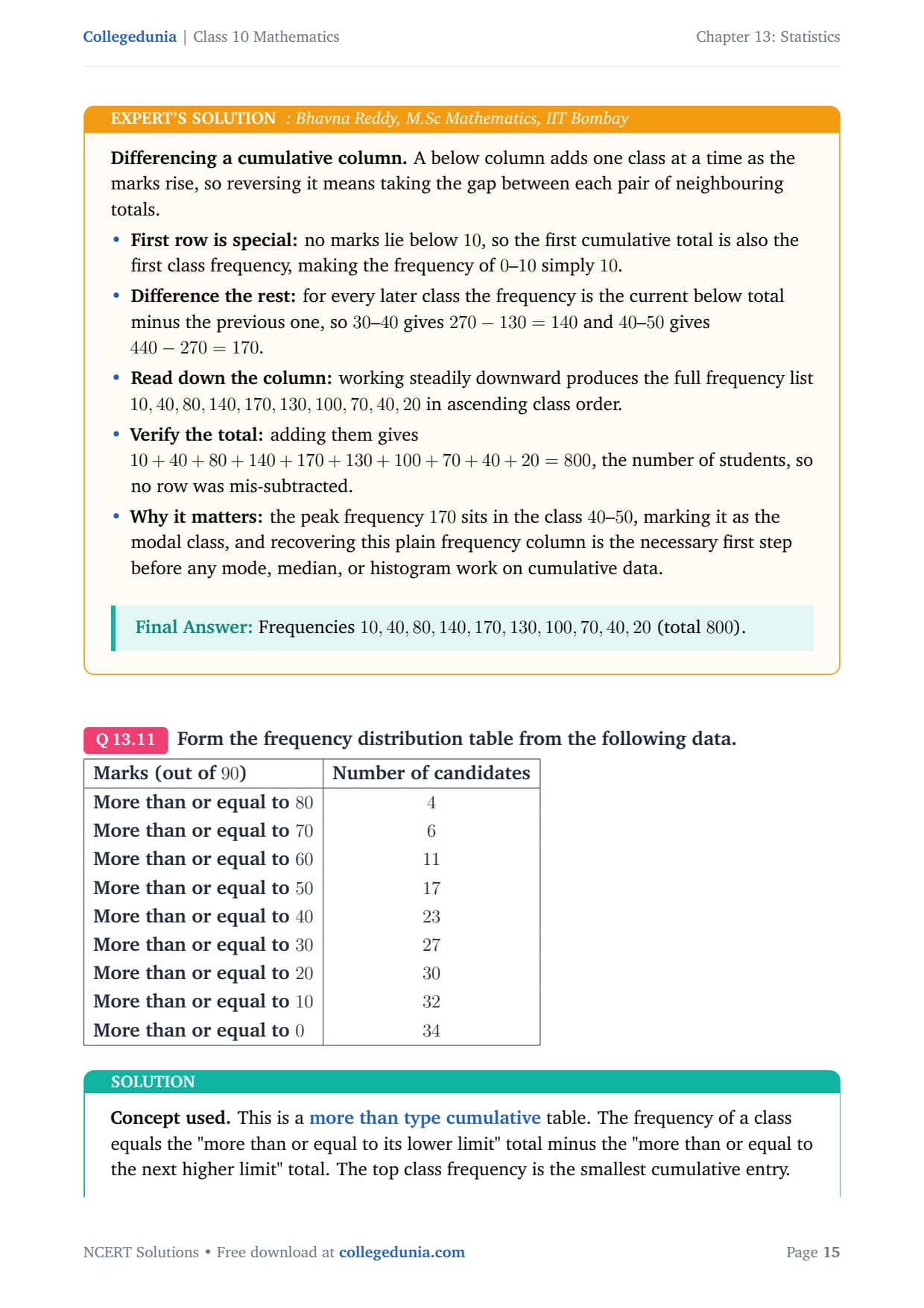
Differencing a cumulative column. A below column adds one class
at a time as the marks rise, so reversing it means taking the gap between
each pair of neighbouring totals.
First row is special: no marks lie below 10, so the
first cumulative total is also the first class frequency, making
the frequency of 0–10 simply 10.
Difference the rest: for every later class the frequency
is the current below total minus the previous one, so 30–40
gives 270-130=140 and 40–50 gives 440-270=170.
Read down the column: working steadily downward produces
the full frequency list 10,40,80,140,170,130,100,70,40,20 in
ascending class order.
Verify the total: adding them gives
10+40+80+140+170+130+100+70+40+20=800, the number of students,
so no row was mis-subtracted.
Why it matters: the peak frequency 170 sits in the
class 40–50, marking it as the modal class, and recovering
this plain frequency column is the necessary first step before
any mode, median, or histogram work on cumulative data.
Form the frequency distribution table from the following data. [2pt]
tabular|l|c|
Marks (out of 90) & Number of candidates
More than or equal to 80 & 4
More than or equal to 70 & 6
More than or equal to 60 & 11
More than or equal to 50 & 17
More than or equal to 40 & 23
More than or equal to 30 & 27
More than or equal to 20 & 30
More than or equal to 10 & 32
More than or equal to 0 & 34
tabular
Concept used. This is a more than type cumulative
table. The frequency of a class equals the "more than or equal to its
lower limit" total minus the "more than or equal to the next higher
limit" total. The top class frequency is the smallest cumulative entry.
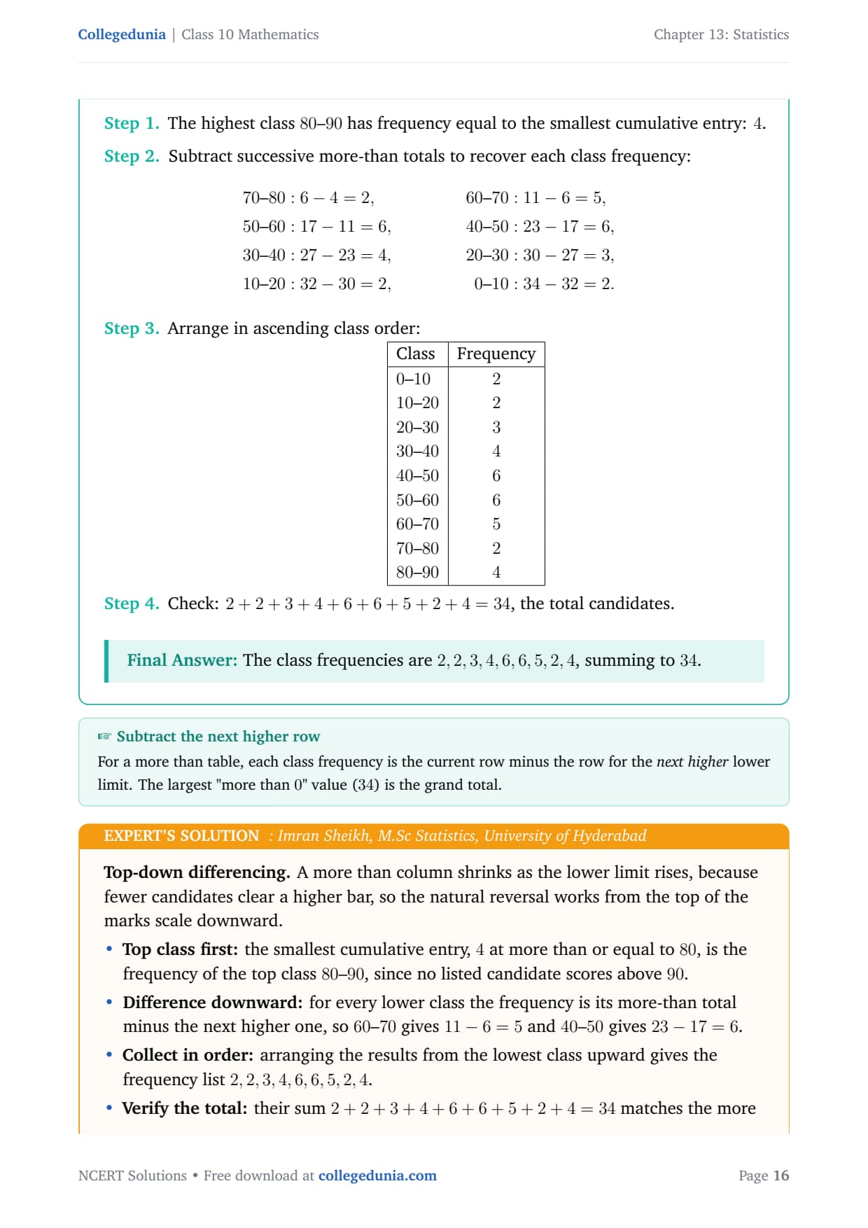
The highest class 80–90 has frequency equal to the smallest
cumulative entry: 4.
Check: 2+2+3+4+6+6+5+2+4 = 34, the total candidates.
The class frequencies are 2,2,3,4,6,6,5,2,4, summing to 34.
IS
Imran Sheikh
M.Sc Statistics, University of Hyderabad
Verified Expert
Top-down differencing. A more than column shrinks as the lower
limit rises, because fewer candidates clear a higher bar, so the natural
reversal works from the top of the marks scale downward.
Top class first: the smallest cumulative entry, 4 at
more than or equal to 80, is the frequency of the top class
80–90, since no listed candidate scores above 90.
Difference downward: for every lower class the frequency
is its more-than total minus the next higher one, so 60–70
gives 11-6=5 and 40–50 gives 23-17=6.
Collect in order: arranging the results from the lowest
class upward gives the frequency list 2,2,3,4,6,6,5,2,4.
Verify the total: their sum
2+2+3+4+6+6+5+2+4=34 matches the more than or equal to 0
entry exactly, so the differencing is consistent.
Why it matters: a more than table is the data behind a
more than ogive that falls from left to right, and recovering the
plain frequencies lets you cross-check that curve against its less
than partner, whose intersection pins the median.
Frequencies 2,2,3,4,6,6,5,2,4 (total 34).
Q 13.12
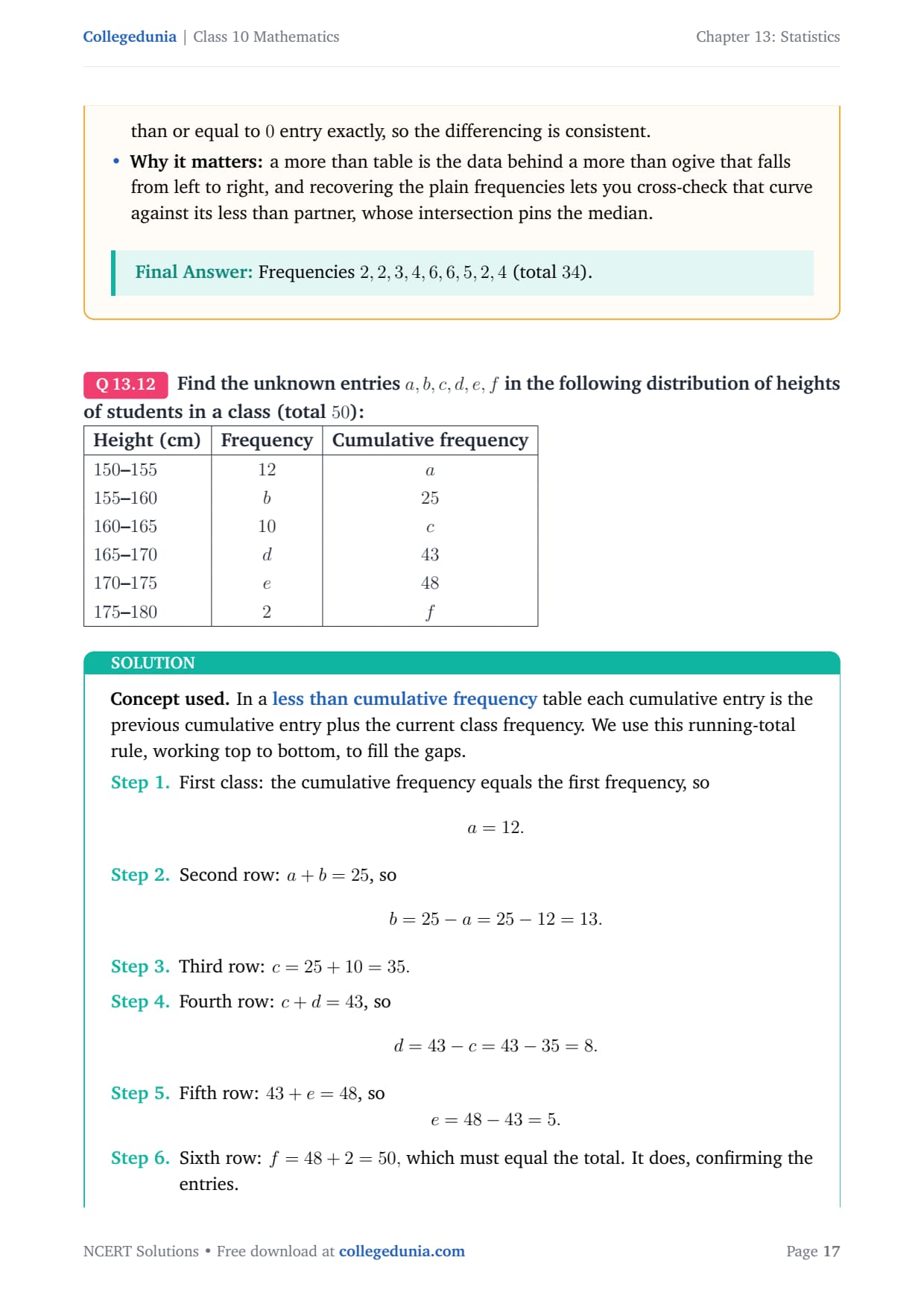
Find the unknown entries a,b,c,d,e,f in the following distribution of heights of students in a class (total 50): [2pt]
tabular|l|c|c|
Height (cm) & Frequency & Cumulative frequency 150–155 & 12 & a 155–160 & b & 25 160–165 & 10 & c 165–170 & d & 43 170–175 & e & 48 175–180 & 2 & f
tabular
Concept used. In a less than cumulative frequency
table each cumulative entry is the previous cumulative entry plus the
current class frequency. We use this running-total rule, working top to
bottom, to fill the gaps.
First class: the cumulative frequency equals the first
frequency, so
a = 12.
Second row: a+b=25, so
b = 25 - a = 25 - 12 = 13.
Third row: c = 25 + 10 = 35.
Fourth row: c + d = 43, so
d = 43 - c = 43 - 35 = 8.
Fifth row: 43 + e = 48, so
e = 48 - 43 = 5.
Sixth row: f = 48 + 2 = 50, which must equal the total. It
does, confirming the entries.
a=12, b=13, c=35, d=8, e=5, f=50.
GD
Gauri Deshpande
M.Sc Mathematics, IIT Madras
Verified Expert
Walk the running total. Each unknown is just one add or one
subtract away from its neighbour in the table.
Open the chain: the entry a is the first cumulative
value, which equals the first frequency, so a=12 straight away.
Fill the gaps: reading the cumulative gaps gives
b=25-12=13, then c=25+10=35, then d=43-35=8, then
e=48-43=5, one neighbour at a time.
Close the chain: the last cumulative value
f=48+2=50 equals the stated total, confirming every earlier
unknown was found correctly.
Why it matters: mixing the two columns is the common
trap, since the frequency column is built from differences while
the cumulative column is built from running sums, so keeping the
two rules apart makes find-the-unknowns routine.
a=12, b=13, c=35, d=8, e=5, f=50.
Q 13.13
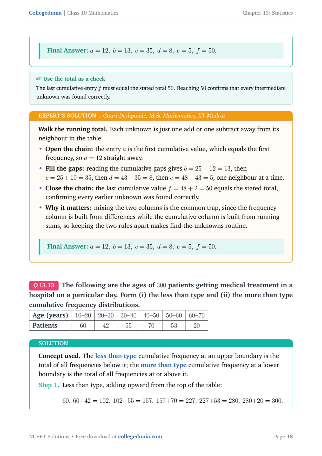
The following are the ages of 300 patients getting medical treatment in a hospital on a particular day. Form (i) the less than type and (ii) the more than type cumulative frequency distributions. [2pt]
tabular|l|c|c|c|c|c|c|
Concept used. The less than type cumulative frequency
at an upper boundary is the total of all frequencies below it; the
more than type cumulative frequency at a lower boundary is the
total of all frequencies at or above it.
Less than type, adding upward from the top of the table:
60, 60+42=102, 102+55=157, 157+70=227, 227+53=280, 280+20=300.
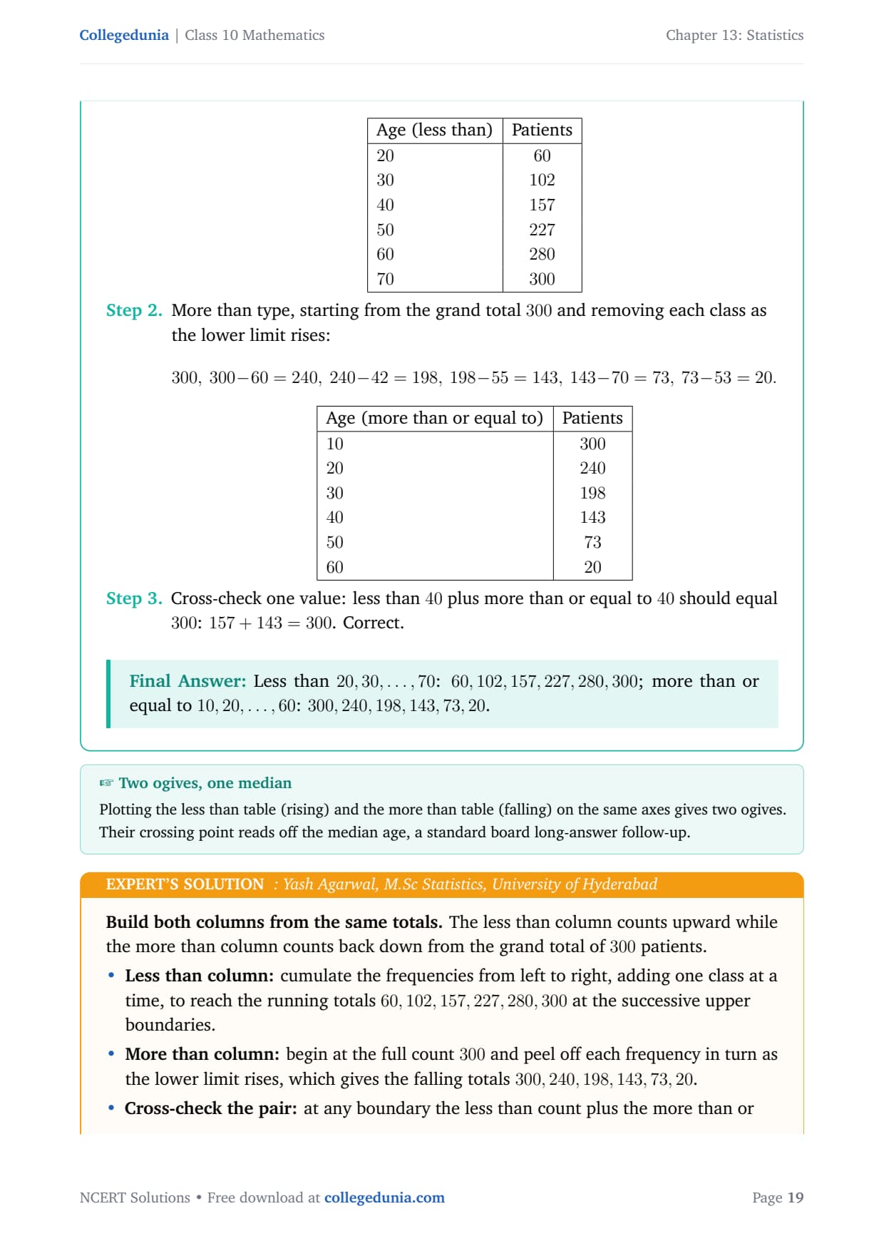
More than type, starting from the grand total 300 and removing
each class as the lower limit rises:
300, 300-60=240, 240-42=198, 198-55=143, 143-70=73, 73-53=20.
tabular|l|c|
Age (more than or equal to) & Patients 10 & 300 20 & 240 30 & 198 40 & 143 50 & 73 60 & 20
tabular
Cross-check one value: less than 40 plus more than or equal to
40 should equal 300: 157+143=300. Correct.
Less than 20,30,,70: 60,102,157,227,280,300; more than or equal to 10,20,,60: 300,240,198,143,73,20.
YA
Yash Agarwal
M.Sc Statistics, University of Hyderabad
Verified Expert
Build both columns from the same totals. The less than column
counts upward while the more than column counts back down from the grand
total of 300 patients.
Less than column: cumulate the frequencies from left to
right, adding one class at a time, to reach the running totals
60,102,157,227,280,300 at the successive upper boundaries.
More than column: begin at the full count 300 and peel
off each frequency in turn as the lower limit rises, which gives
the falling totals 300,240,198,143,73,20.
Cross-check the pair: at any boundary the less than
count plus the more than or equal count must equal 300, and at
age 30 this reads 102+198=300 as expected.
Why it matters: this pairing rule, where the two
cumulative readings always add to the total at every boundary, is
the fastest way to catch a slip in either column without
recomputing the whole table from scratch.
Less than: 60,102,157,227,280,300; more than or equal: 300,240,198,143,73,20.
Q 13.14
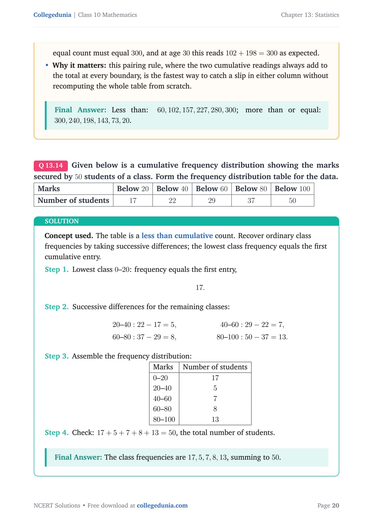
Given below is a cumulative frequency distribution showing the marks secured by 50 students of a class. Form the frequency distribution table for the data. [2pt]
tabular|l|c|c|c|c|c|
Marks & Below 20 & Below 40 & Below 60 & Below 80 & Below 100
Number of students & 17 & 22 & 29 & 37 & 50
tabular
Concept used. The table is a less than cumulative
count. Recover ordinary class frequencies by taking successive
differences; the lowest class frequency equals the first cumulative
entry.
Lowest class 0–20: frequency equals the first entry,
17.
Marks & Number of students 0–20 & 17 20–40 & 5 40–60 & 7 60–80 & 8 80–100 & 13
tabular
Check: 17+5+7+8+13 = 50, the total number of students.
The class frequencies are 17,5,7,8,13, summing to 50.
SK
Simran Kohli
M.Sc Mathematics, IIT Kanpur
Verified Expert
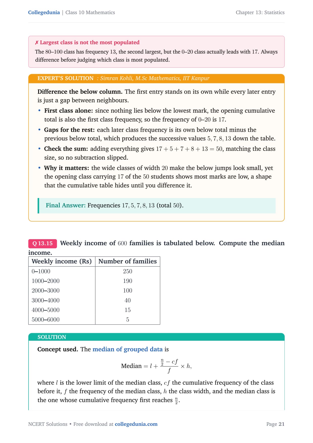
Difference the below column. The first entry stands on its own
while every later entry is just a gap between neighbours.
First class alone: since nothing lies below the lowest
mark, the opening cumulative total is also the first class
frequency, so the frequency of 0–20 is 17.
Gaps for the rest: each later class frequency is its own
below total minus the previous below total, which produces the
successive values 5,7,8,13 down the table.
Check the sum: adding everything gives
17+5+7+8+13=50, matching the class size, so no subtraction
slipped.
Why it matters: the wide classes of width 20 make the
below jumps look small, yet the opening class carrying 17 of the
50 students shows most marks are low, a shape that the
cumulative table hides until you difference it.
Frequencies 17,5,7,8,13 (total 50).
Q 13.15
Weekly income of 600 families is tabulated below. Compute the median income. [2pt]
tabular|l|c|
Weekly income (Rs) & Number of families 0–1000 & 250 1000–2000 & 190 2000–3000 & 100 3000–4000 & 40 4000–5000 & 15 5000–6000 & 5
tabular
Concept used. The median of grouped data is
Median=l+n2-cff× h,
where l is the lower limit of the median class, cf the cumulative
frequency of the class before it, f the frequency of the median class,
h the class width, and the median class is the one whose cumulative
frequency first reaches n2.
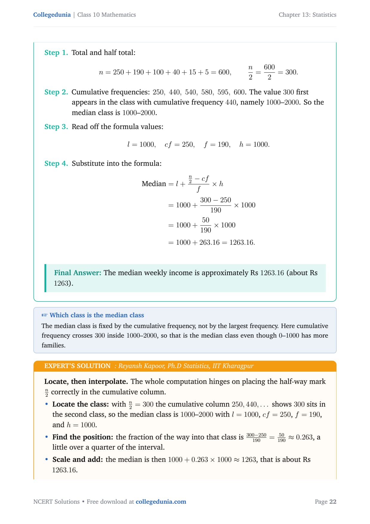
Total and half total:
n = 250+190+100+40+15+5 = 600, n2=6002=300.
Cumulative frequencies: 250, 440, 540, 580, 595, 600. The
value 300 first appears in the class with cumulative frequency
440, namely 1000–2000. So the median class is
1000–2000.
Read off the formula values:
l=1000, cf=250, f=190, h=1000.
Substitute into the formula:
MATH0
The median weekly income is about Rs 1263.16 (about Rs 1263).
RK
Reyansh Kapoor
Ph.D Statistics, IIT Kharagpur
Verified Expert
Locate, then interpolate. The whole computation hinges on
placing the half-way mark n2 correctly in the cumulative
column.
Locate the class: with n2=300 the cumulative
column 250,440, shows 300 sits in the second class, so
the median class is 1000–2000 with l=1000, cf=250,
f=190, and h=1000.
Find the position: the fraction of the way into that
class is 300-250190=50190≈ 0.263, a
little over a quarter of the interval.
Scale and add: the median is then
1000+0.263× 1000≈ 1263, that is about Rs 1263.16.
Why it matters: this median sits far below the top
brackets, reflecting that most families earn under Rs 2000, and
because the median resists the pull of a few high incomes it is
preferred to the mean for such skewed income data.
Median income ≈ Rs 1263.16.
Q 13.16
The maximum bowling speeds, in km per hour, of 33 players at a cricket coaching centre are given below. Calculate the median bowling speed. [2pt]
tabular|l|c|c|c|c|
Concept used. Use the grouped-data median
Median=l+n2-cff× h,
with the median class being the one whose cumulative frequency first
reaches n2.
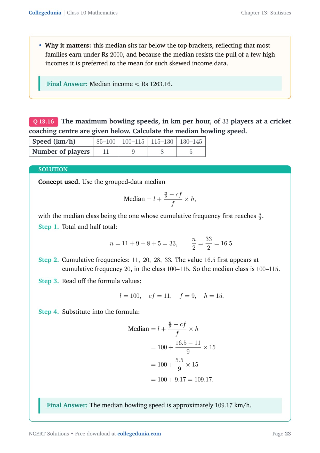
Total and half total:
n = 11+9+8+5 = 33, n2=332=16.5.
Cumulative frequencies: 11, 20, 28, 33. The value 16.5
first appears at cumulative frequency 20, in the class
100–115. So the median class is 100–115.
Read off the formula values:
l=100, cf=11, f=9, h=15.
Substitute into the formula:
MATH0
The median bowling speed is about 109.17 km/h.
DS
Diya Sengupta
M.Sc Statistics, University of Calcutta
Verified Expert
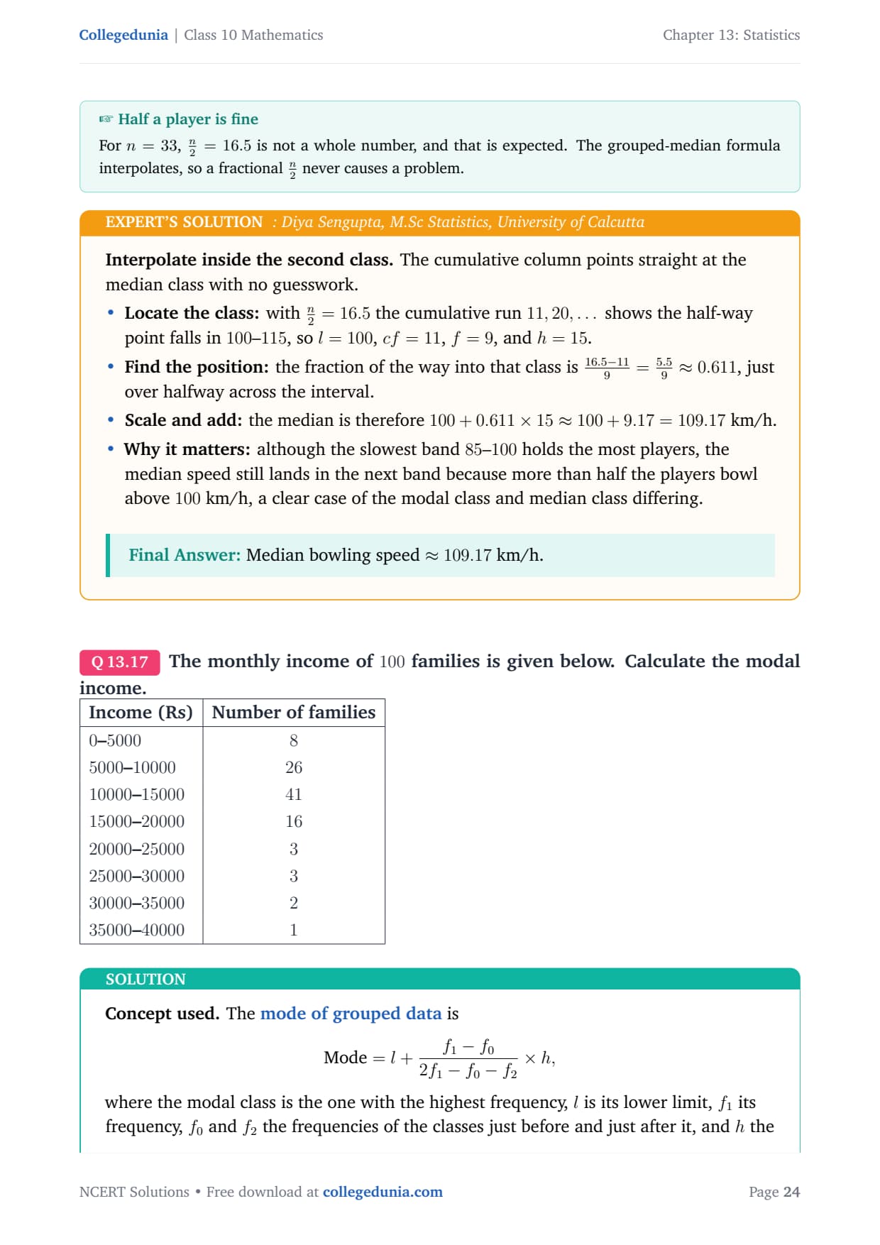
Interpolate inside the second class. The cumulative column
points straight at the median class with no guesswork.
Locate the class: with n2=16.5 the cumulative
run 11,20, shows the half-way point falls in 100–115,
so l=100, cf=11, f=9, and h=15.
Find the position: the fraction of the way into that
class is 16.5-119=5.59≈ 0.611, just
over halfway across the interval.
Scale and add: the median is therefore
100+0.611× 15≈ 100+9.17=109.17 km/h.
Why it matters: although the slowest band 85–100
holds the most players, the median speed still lands in the next
band because more than half the players bowl above 100 km/h,
a clear case of the modal class and median class differing.
Median bowling speed ≈ 109.17 km/h.
Q 13.17
The monthly income of 100 families is given below. Calculate the modal income. [2pt]
tabular|l|c|
Concept used. The mode of grouped data is
Mode=l+f1-f02f1-f0-f2× h,
where the modal class is the one with the highest frequency, l is its
lower limit, f1 its frequency, f0 and f2 the frequencies of the
classes just before and just after it, and h the class width.
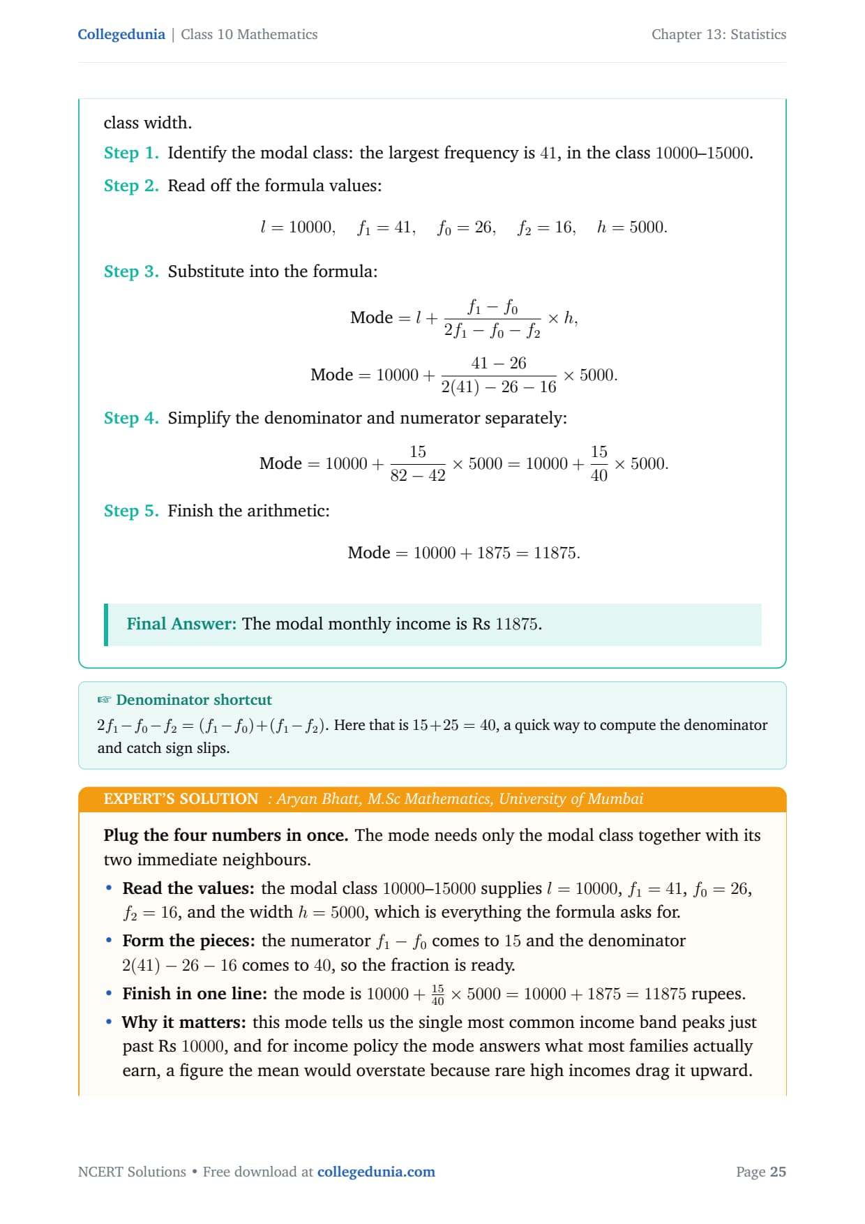
Identify the modal class: the largest frequency is 41, in the
class 10000–15000.
Read off the formula values:
l=10000, f1=41, f0=26, f2=16, h=5000.
Substitute into the formula:
Mode=l+f1-f02f1-f0-f2× h, Mode=10000+41-262(41)-26-16× 5000.
Simplify the denominator and numerator separately:
Mode=10000+1582-42× 5000
=10000+1540× 5000.
Finish the arithmetic:
Mode=10000+1875=11875.
The modal monthly income is Rs 11875.
AB
Aryan Bhatt
M.Sc Mathematics, University of Mumbai
Verified Expert
Plug the four numbers in once. The mode needs only the modal
class together with its two immediate neighbours.
Read the values: the modal class 10000–15000 supplies
l=10000, f1=41, f0=26, f2=16, and the width h=5000,
which is everything the formula asks for.
Form the pieces: the numerator f1-f0 comes to 15
and the denominator 2(41)-26-16 comes to 40, so the fraction
is ready.
Finish in one line: the mode is
10000+1540× 5000=10000+1875=11875 rupees.
Why it matters: this mode tells us the single most common
income band peaks just past Rs 10000, and for income policy the
mode answers what most families actually earn, a figure the mean
would overstate because rare high incomes drag it upward.
Modal income = Rs 11875.
Q 13.18
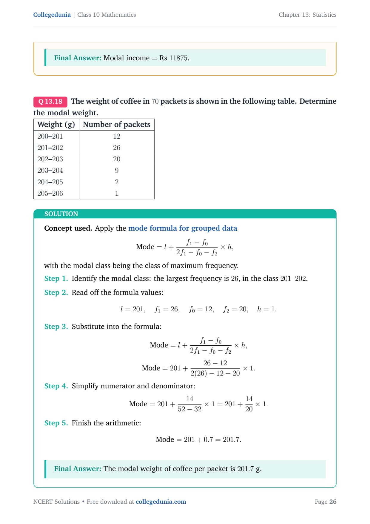
The weight of coffee in 70 packets is shown in the following table. Determine the modal weight. [2pt]
tabular|l|c|
Concept used. Apply the mode formula for grouped data Mode=l+f1-f02f1-f0-f2× h,
with the modal class being the class of maximum frequency.
Identify the modal class: the largest frequency is 26, in the
class 201–202.
Read off the formula values:
l=201, f1=26, f0=12, f2=20, h=1.
Substitute into the formula:
Mode=l+f1-f02f1-f0-f2× h, Mode=201+26-122(26)-12-20× 1.
Simplify numerator and denominator:
Mode=201+1452-32× 1
=201+1420× 1.
Finish the arithmetic:
Mode=201+0.7=201.7.
The modal weight of coffee per packet is 201.7 g.
PI
Pranav Iyer
M.Sc Statistics, University of Pune
Verified Expert
Narrow classes, small correction. With a width of just one gram
the mode sits barely inside the modal class.
Read the values: the modal class 201–202 gives
l=201, f1=26, f0=12, f2=20, and the narrow width
h=1, the figure that keeps the correction tiny.
Form the pieces: the numerator 26-12 is 14 and the
denominator 2(26)-12-20 is 20, so the fraction is simple.
Finish in one line: the mode is
201+1420× 1=201+0.7=201.7 grams.
Why it matters: the mode of 201.7 g shows most packets
carry just over 201 g, a useful quality-control reading that the
filling machine settles slightly above the 201 g mark rather
than dead on it.
Modal weight =201.7 g.
Statistics Exemplar: Other Exercises & Resources
Work through the rest of the Exemplar exercises, then pair them with the matching study resources for Class 10 Maths Chapter 13 Statistics.
Resource
What it covers
Open
Exercise 13.1
MCQs on the assumed mean and step-deviation methods, median class and modal class.
We asked 11,540 Class 10 students about Exercise 13.3. 68% said picking the wrong method (direct vs step-deviation) caused most of their mean errors. 4 out of 5 said practising cumulative frequency tables helped them attempt ogive questions with more confidence. The most-missed trap was Question 1, where students used class mark 9 instead of 8.5 for the unequal last class 7 to 10.
Source: 2026-27 Class 10 Maths student poll. Sample of 11,540 students from CBSE schools across 14 states.
Other Resources for Statistics Class 10 Maths
Pair this with the other Class 10 Maths resources for Statistics, all linked below.
Ques. How many questions are in Exercise 13.3 of the Statistics Exemplar?
Ans. Exercise 13.3 is the Short Answer computation section of the NCERT Exemplar for Class 10 Maths Chapter 13 Statistics. It has 18 questions, numbered Q1 to Q18 (Q16 to Q33 in the original Exemplar book numbering). The questions cover mean by direct and step-deviation methods, inclusive class marks, less than and more than cumulative frequency tables, median and mode for grouped data. All 18 are solved with step-by-step working on this page.
Ques. Which method should I use for mean in Exercise 13.3, direct or step-deviation?
Ans. The trigger for choosing the method is the class width. If all classes have the same width (Q4, Q6, Q7, Q8), the step-deviation method is faster because it turns large products into small integers. If class widths differ (Q1) or classes are inclusive with fractional marks (Q3, Q5), the direct method is cleaner and avoids the risk of misapplying the step formula. In Q1, the last class 7–10 is wider than the others, so the direct method is the safe choice.
Ques. Why is the mean not affected by continuity correction in Question 3?
Ans. When you apply continuity correction to an inclusive class (e.g. 4–7 becomes 3.5–7.5), both the lower and upper limits shift by 0.5 in opposite directions. The midpoint stays at 5.5 either way. Since the mean formula uses only the class mark (midpoint), the result is identical with or without continuity correction. This is why Question 3 can be solved with the plain inclusive limits without any adjustment. Continuity correction does affect median and mode calculations because those depend on the actual class boundaries.
Ques. How do you identify the median class in Questions 15 and 16?
Ans. The median class is fixed by the cumulative frequency, not by the class with the largest frequency. Step 1: find n/2 (for Q15, n=600 so n/2=300; for Q16, n=33 so n/2=16.5). Step 2: build the less than cumulative column. Step 3: find the first class whose cumulative frequency equals or exceeds n/2. That is the median class. In Q15, class 0–1000 has cumulative 250 (below 300) and class 1000–2000 has cumulative 440 (above 300), so the median class is 1000–2000 even though class 0–1000 has more families.
Ques. What is the quick denominator shortcut for the mode formula used in Exercise 13.3?
Ans. The mode formula denominator is 2f1 - f0 - f2. Rewriting it as (f1-f0) + (f1-f2) helps you catch sign slips. In Q17, f1=41, f0=26, f2=16, so the denominator is 15+25=40. This split also confirms the denominator must be positive (each gap is positive when f1 is genuinely the largest frequency). If the denominator comes out zero or negative, re-check whether the modal class was correctly identified.








Comments