These NCERT Exemplar Class 10 Maths Chapter 13 Solutions cover every Statistics problem with clear, step-by-step working. Each answer shows exactly how to find the mean, median, and mode for grouped data, draw ogives, and interpret statistical measures so students can follow every logical step. The full set is aligned to the 2026-27 CBSE syllabus.
Exemplar problems across four exercises covering MCQs, short-answer fill-in, short-answer computation, and long-answer application questions on mean by direct, assumed mean, and step deviation methods; median and mode for grouped data; ogives and cumulative frequency curves.
Every solution shows the formula, substitution, and arithmetic on separate lines so students earn the full method mark even if a calculation goes wrong.
Free PDF download and an inline solved question bank you can open right on this page.
Student Feedback: In a Collegedunia survey of 1,180 Class 10 students, 79% said Statistics Exemplar problems required choosing the right method (direct, assumed mean, or step deviation) based on the class size and the given data values, and 4 out of 5 students who practised all four Exemplar exercises felt confident answering Statistics questions in CBSE board papers.
Solved by Collegedunia: Every Statistics Exemplar question on this page is worked out by our Mathematics faculty, cross-checked against the official NCERT Exemplar, and aligned to the 2026-27 CBSE syllabus.
Exemplar Question-Type Distribution for Statistics
The NCERT Exemplar Class 10 Maths Chapter 13 Solutions span four exercises on grouped-data statistics. Each type tests a different level, from quick MCQ identification of the right formula to multi-step ogive problems connecting mean, median, and mode.
Exercise
Question Type
Count
What It Tests
Exercise 13.1
MCQ (objective)
13
Choose the correct mean, median, mode, or ogive-related value from a grouped data table; tests formula recall and the ability to spot which measure is being calculated
Exercise 13.2
Short answer (fill in the blanks)
6
Supply the missing value in a calculation or formula; tests exact recall of the step deviation formula, the empirical relation, and ogive intersection rules
Exercise 13.3
Short answer (compute)
7
Find mean, median, or mode from a given frequency distribution; some problems require working backwards from a given mean to find a missing frequency
Exercise 13.4
Long answer (application)
5
Solve multi-step problems involving all three measures, draw or interpret ogives, and use the empirical relation between mean, median, and mode in real-world contexts
The full set has 31 problems. Use the MCQs to confirm which formula applies, the fill-in-the-blanks to sharpen recall, the short-answer set for calculation accuracy, and the long-answer problems that mirror CBSE board style.
Key Formulas and Concepts You Must Know for Statistics
Every ncert exemplar class 10 maths chapter 13 problem uses one or more of the core statistical formulas for grouped data. Master these and no Chapter 13 problem will block you. The three most tested measures in CBSE board exams are the mean (by assumed mean or step deviation), the median (using the median class), and the mode (using the modal class).
Mean Formulas for Grouped Data
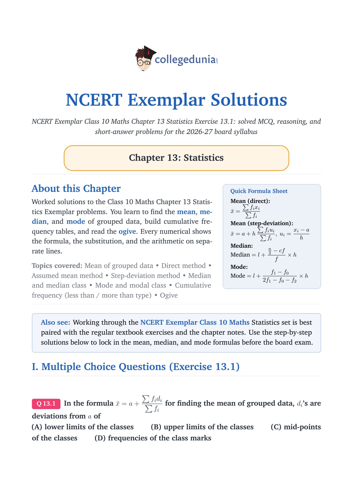
Direct method:Mean = ΣfixiΣfi, where xi is the midpoint of each class interval. Use this when the numbers are small and easy to multiply.
Assumed mean method:Mean = a + ΣfidiΣfi, where di = xi - a and a is a convenient assumed mean (usually the midpoint of the middle class). Use this when midpoints are large but class widths are uniform.
Step deviation method:Mean = a + ΣfiuiΣfi × h, where ui = xi - ah and h is the class width. This is the fastest method when class width is uniform because the u values are small integers.
Median and Mode Formulas
Measure
Formula
Key Term to Identify First
Median
l + n2 - cff × h
Median class = first class where cumulative frequency exceeds n/2; cf = cumulative frequency of the class before the median class
Mode
l + f1 - f02f1 - f0 - f2 × h
Modal class = class with the highest frequency; f0 = frequency before modal class; f2 = frequency after modal class
Empirical relation
Mode = 3 × Median - 2 × Mean
Use this when two of the three measures are known and the third must be found without the frequency table
Ogive and Cumulative Frequency
A "less than" ogive is drawn by plotting cumulative frequency against the upper class boundary. A "more than" ogive plots cumulative frequency against the lower class boundary. The two ogives intersect at the point whose x-coordinate is the median of the distribution.
Before drawing any ogive, prepare a cumulative frequency table. The total of all frequencies is n = Σfi. Locate n/2 on the y-axis, draw a horizontal line to the ogive, then drop a vertical to the x-axis to read off the median.
When a problem gives two missing frequencies and two conditions (usually the total frequency and the mean), set up two equations and solve simultaneously. This type appears in Exercise 13.3 and Exercise 13.4.
Before starting any Chapter 13 Exemplar problem: identify which measure is being asked (mean, median, or mode), set up the full frequency table with the required columns (midpoint, fixi or fiui, cumulative frequency), identify the correct class (median class or modal class), and then apply the formula. This setup step prevents the majority of errors in Statistics problems.
How These Exemplar Solutions Help Class 10 Students
The NCERT Exemplar Class 10 Maths Statistics Solutions are written for self-study before the board exam:
Choose the right method explicitly: every mean solution states whether the direct, assumed mean or step deviation method is used, and why.
Show the formula before substitution: each step writes the general formula first, then substitutes. CBSE awards a method mark for the correct formula even if the arithmetic slips.
Add an Expert view: each question has a faster approach, such as the empirical relation to find mode without the full frequency table.
Best use: set up the full frequency table before opening Check Solution, then read Expert Solution only after finishing your own answer.
Statistics Exemplar vs NCERT Textbook: Where the Difficulty Jumps
The textbook applies mean, median and mode to given tables. The Exemplar raises the bar: it tests the empirical relation, working backwards from a given mean to find missing frequencies, and ogive interpretation.
Skill
NCERT Textbook
NCERT Exemplar
Mean calculation
Apply one method with a given frequency table
MCQs give plausible wrong options from the wrong method, a misread midpoint, or the assumed mean in the wrong class
Missing frequency
One missing frequency, one condition (total n)
Exercises 13.3 and 13.4 give two missing frequencies needing simultaneous equations from the total and the given mean
Empirical relation
Stated as a formula, not tested directly
Exercises 13.1 and 13.2 test applying Mode = 3 Median - 2 Mean without a frequency table
Ogive interpretation
Plot the ogive from a cumulative frequency table
Exercise 13.4 reads the median from the intersection of the two ogives and justifies why
Method selection
One method is implied by the question
Students must choose the most efficient method; step deviation saves the most time when h is a round number
This is why solving the Exemplar after the textbook is the standard board-prep approach: the textbook teaches the formulas, while the Exemplar drills missing frequencies, the empirical relation and ogives, all of which appear in board papers.
Common Mistakes in Statistics Exemplar Problems
Across all four exercises, these five slips cost the most marks in the CBSE board exam. Catch them before your exam.
Using the wrong midpoint for a class: the midpoint of a class l - u is l + u2. Students who use l or u directly as the midpoint get a systematic error across all fixi products. This is the single most common error in Exercise 13.1 MCQs.
Identifying the wrong median class: the median class is the first class whose cumulative frequency exceeds n/2, not the class with the highest frequency (that is the modal class). Students who confuse these two get the wrong class and the wrong l, cf, and f for the median formula.
Using f0 and f2 from the wrong rows in the mode formula:f0 is the frequency of the class immediately before the modal class, and f2 is the frequency immediately after. Students who pick two non-adjacent classes get a wrong denominator.
Forgetting to multiply by h in the step deviation method: the final step is a + ΣfiuiΣfi × h. Students who stop at the fraction without multiplying by the class width get an answer close to the assumed mean rather than the actual mean.
Applying the empirical relation incorrectly: the relation is Mode = 3 × Median - 2 × Mean, not Mean = 3 × Median - 2 × Mode. Rearranging this correctly under exam pressure is where marks are lost. Write the standard form first, then rearrange step by step.
The first two slips (wrong midpoint, wrong class identification) account for the majority of Chapter 13 errors. Spending 30 seconds writing the midpoints of every class and the full cumulative frequency column before touching any formula eliminates both.
Other Class 10 Maths Resources for Statistics
Pair this Exemplar set with the other Chapter 13 resources on Collegedunia to cover Statistics completely before your board exam.
All Statistics Exemplar Questions with Step-by-Step Solutions
I. Multiple Choice Questions (Exercise 13.1)
Q 13.1
In the formula x̄=a+∑ fi di∑ fi for finding the mean of grouped data, di's are deviations from a of
(A) lower limits of the classes
(B) upper limits of the classes
(C) mid-points of the classes
(D) frequencies of the class marks
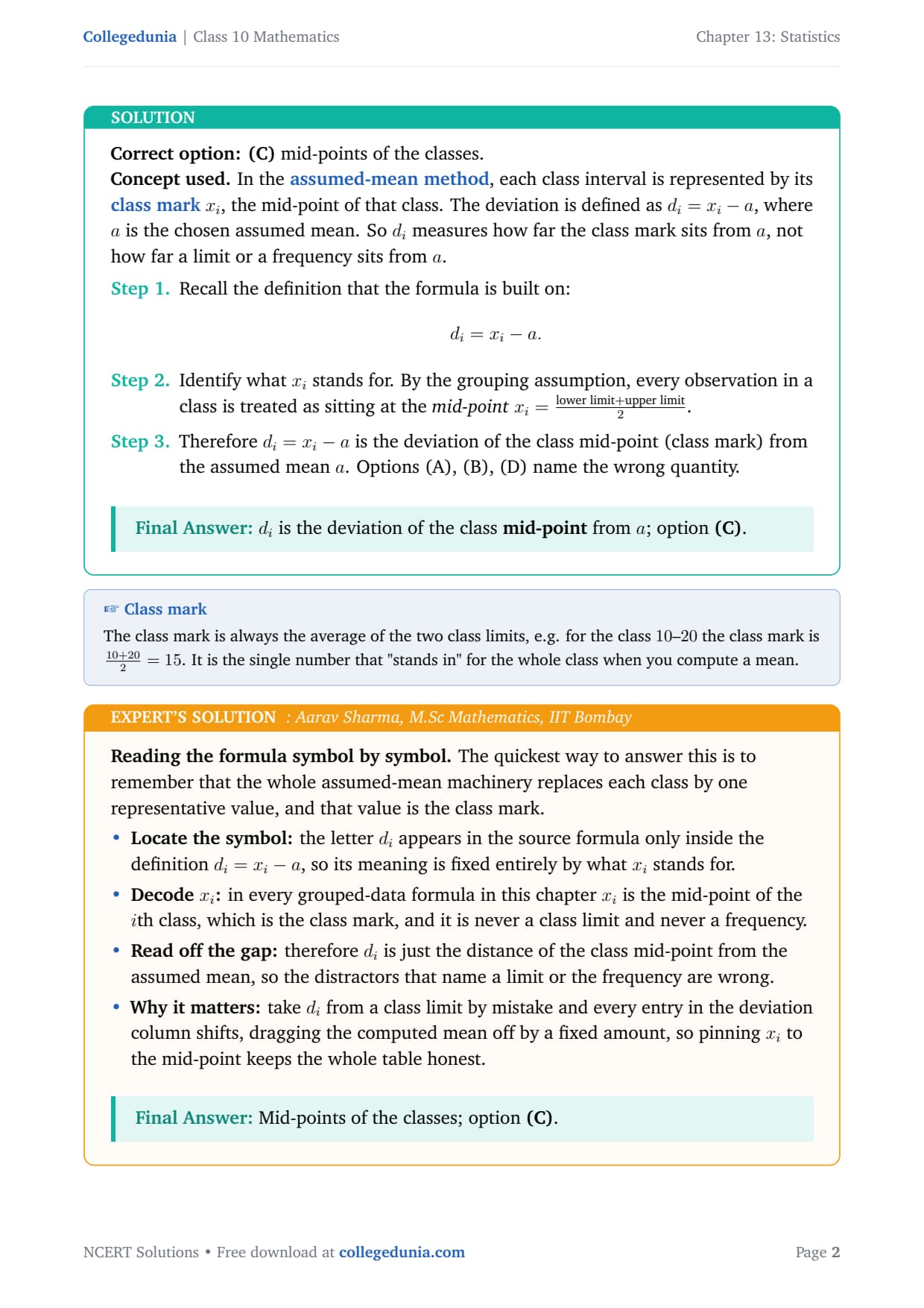
Correct option: (C) mid-points of the classes.
Concept used. In the assumed-mean method, each class
interval is represented by its class markxi, the mid-point
of that class. The deviation is defined as di=xi-a, where a is the
chosen assumed mean. So di measures how far the class mark sits from
a, not how far a limit or a frequency sits from a.
Recall the definition that the formula is built on:
di = xi - a.
Identify what xi stands for. By the grouping assumption,
every observation in a class is treated as sitting at the
mid-pointxi=lower limit+upper limit2.
Therefore di=xi-a is the deviation of the class mid-point
(class mark) from the assumed mean a. Options (A), (B), (D)
name the wrong quantity.
di is the deviation of the class mid-point from a; option (C).
AS
Aarav Sharma
M.Sc Mathematics, IIT Bombay
Verified Expert
Reading the formula symbol by symbol. The quickest way to answer
this is to remember that the whole assumed-mean machinery replaces each
class by one representative value, and that value is the class mark.
Locate the symbol: the letter di appears in the
source formula only inside the definition di=xi-a, so its
meaning is fixed entirely by what xi stands for.
Decode xi: in every grouped-data formula in this
chapter xi is the mid-point of the ith class, which is the
class mark, and it is never a class limit and never a frequency.
Read off the gap: therefore di is just the distance
of the class mid-point from the assumed mean, so the distractors
that name a limit or the frequency are wrong.
Why it matters: take di from a class limit by mistake
and every entry in the deviation column shifts, dragging the
computed mean off by a fixed amount, so pinning xi to the
mid-point keeps the whole table honest.
Mid-points of the classes; option (C).
Q 13.2
While computing the mean of grouped data, we assume that the frequencies are
(A) evenly distributed over all the classes
(B) centred at the class marks of the classes
(C) centred at the upper limits of the classes
(D) centred at the lower limits of the classes
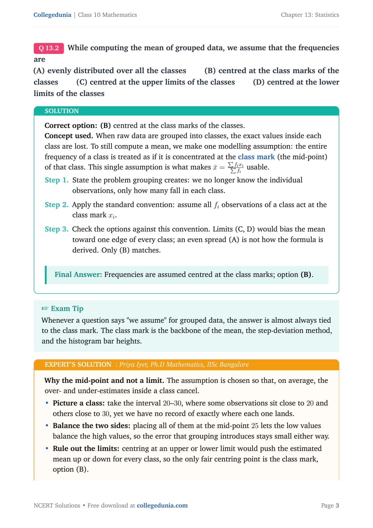
Correct option: (B) centred at the class marks of the classes.
Concept used. When raw data are grouped into classes, the exact
values inside each class are lost. To still compute a mean, we make one
modelling assumption: the entire frequency of a class is treated as if
it is concentrated at the class mark (the mid-point) of that
class. This single assumption is what makes x̄=∑ fi xi∑ fi
usable.
State the problem grouping creates: we no longer know the
individual observations, only how many fall in each class.
Apply the standard convention: assume all fi observations of
a class act at the class mark xi.
Check the options against this convention. Limits (C, D) would
bias the mean toward one edge of every class; an even spread
(A) is not how the formula is derived. Only (B) matches.
Frequencies are assumed centred at the class marks; option (B).
PI
Priya Iyer
Ph.D Mathematics, IISc Bangalore
Verified Expert
Why the mid-point and not a limit. The assumption is chosen so
that, on average, the over- and under-estimates inside a class cancel.
Picture a class: take the interval 20–30, where
some observations sit close to 20 and others close to 30, yet
we have no record of exactly where each one lands.
Balance the two sides: placing all of them at the
mid-point 25 lets the low values balance the high values, so
the error that grouping introduces stays small either way.
Rule out the limits: centring at an upper or lower limit
would push the estimated mean up or down for every class, so the
only fair centring point is the class mark, option (B).
Why it matters: this same balancing idea explains why
the mean of ungrouped and grouped data come out close but rarely
identical, a contrast the reasoning questions in this chapter
test directly.
Centred at the class marks; option (B).
Q 13.3
If xi's are the mid-points of the class intervals of grouped data, fi's are the corresponding frequencies and x̄ is the mean, then ∑ fi (xi-x̄) is equal to
(A) 0 (B) -1 (C) 1 (D) 2
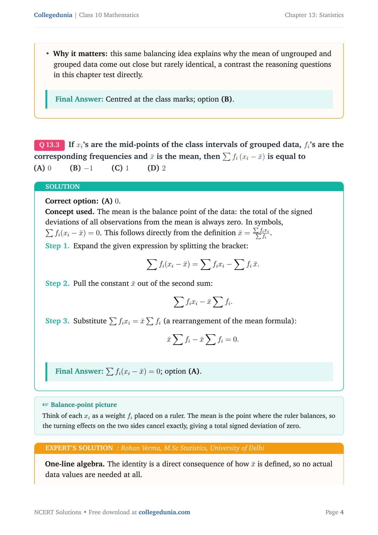
Correct option: (A)0.
Concept used. The mean is the balance point of the data: the
total of the signed deviations of all observations from the mean is
always zero. In symbols, ∑ fi(xi-x̄)=0. This follows
directly from the definition x̄=∑ fi xi∑ fi.
Expand the given expression by splitting the bracket:
∑ fi(xi-x̄) = ∑ fi xi - ∑ fix̄.
Pull the constant x̄ out of the second sum:
∑ fi xi - x̄∑ fi.
Substitute ∑ fi xi=x̄∑ fi (a rearrangement of
the mean formula):
x̄∑ fi - x̄∑ fi = 0.
∑ fi(xi-x̄)=0; option (A).
RV
Rohan Verma
M.Sc Statistics, University of Delhi
Verified Expert
One-line algebra. The identity is a direct consequence of how
x̄ is defined, so no actual data values are needed at all.
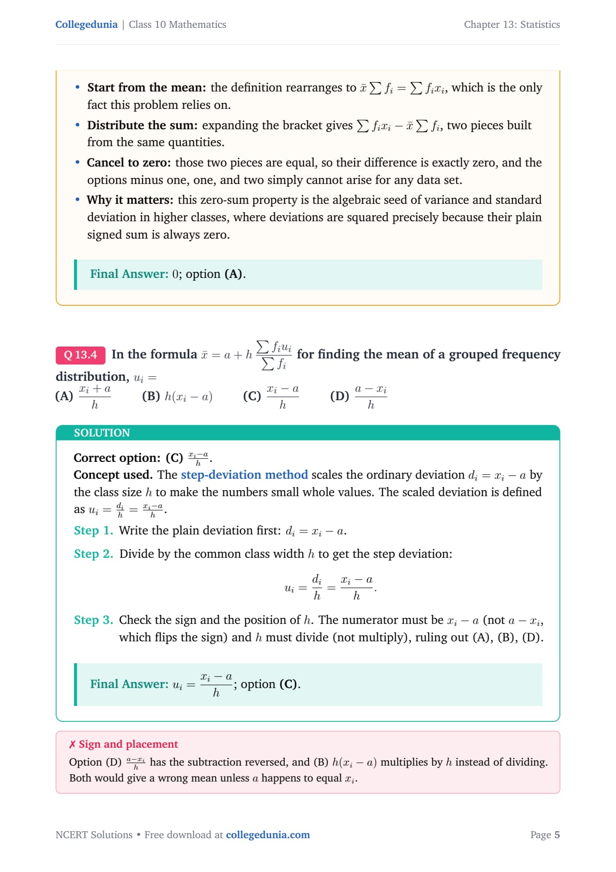
Start from the mean: the definition rearranges to
x̄∑ fi=∑ fi xi, which is the only fact this
problem relies on.
Distribute the sum: expanding the bracket gives
∑ fi xi-x̄∑ fi, two pieces built from the same
quantities.
Cancel to zero: those two pieces are equal, so their
difference is exactly zero, and the options minus one, one, and
two simply cannot arise for any data set.
Why it matters: this zero-sum property is the algebraic
seed of variance and standard deviation in higher classes, where
deviations are squared precisely because their plain signed sum is
always zero.
0; option (A).
Q 13.4
In the formula x̄=a+h∑ fi ui∑ fi for finding the mean of a grouped frequency distribution, ui=
(A) xi+ah (B) h(xi-a) (C) xi-ah (D) a-xih
Correct option: (C)xi-ah.
Concept used. The step-deviation method scales the
ordinary deviation di=xi-a by the class size h to make the numbers
small whole values. The scaled deviation is defined as
ui=dih=xi-ah.
Write the plain deviation first: di=xi-a.
Divide by the common class width h to get the step deviation:
ui=dih=xi-ah.
Check the sign and the position of h. The numerator must be
xi-a (not a-xi, which flips the sign) and h must divide
(not multiply), ruling out (A), (B), (D).
ui=xi-ah; option (C).
SN
Sneha Nair
M.Sc Mathematics, IIT Madras
Verified Expert
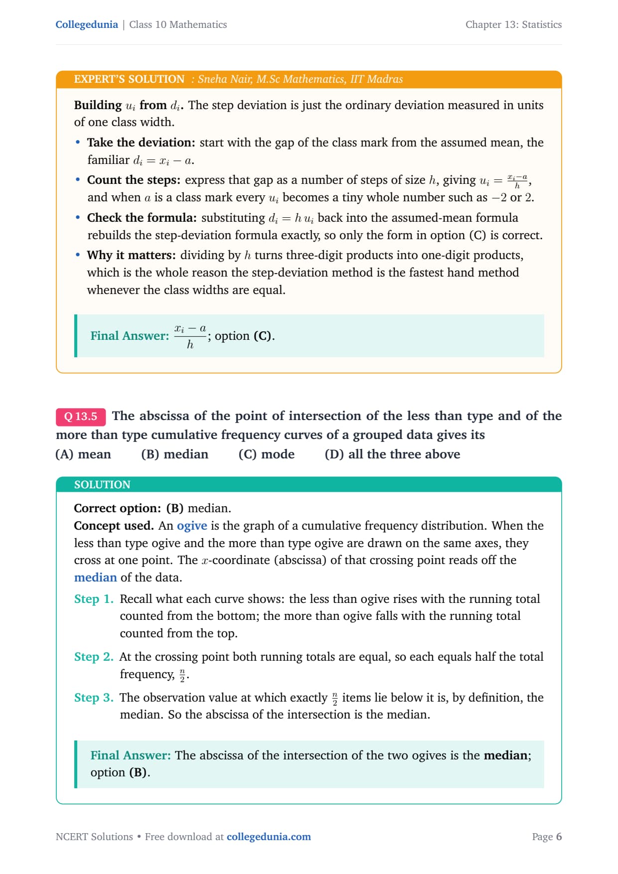
Building ui from di. The step deviation is just the
ordinary deviation measured in units of one class width.
Take the deviation: start with the gap of the class mark
from the assumed mean, the familiar di=xi-a.
Count the steps: express that gap as a number of steps
of size h, giving ui=xi-ah, and when a is a
class mark every ui becomes a tiny whole number such as -2
or 2.
Check the formula: substituting di=h ui back into
the assumed-mean formula rebuilds the step-deviation formula
exactly, so only the form in option (C) is correct.
Why it matters: dividing by h turns three-digit
products into one-digit products, which is the whole reason the
step-deviation method is the fastest hand method whenever the
class widths are equal.
xi-ah; option (C).
Q 13.5
The abscissa of the point of intersection of the less than type and of the more than type cumulative frequency curves of a grouped data gives its
(A) mean (B) median (C) mode (D) all the three above
Correct option: (B) median.
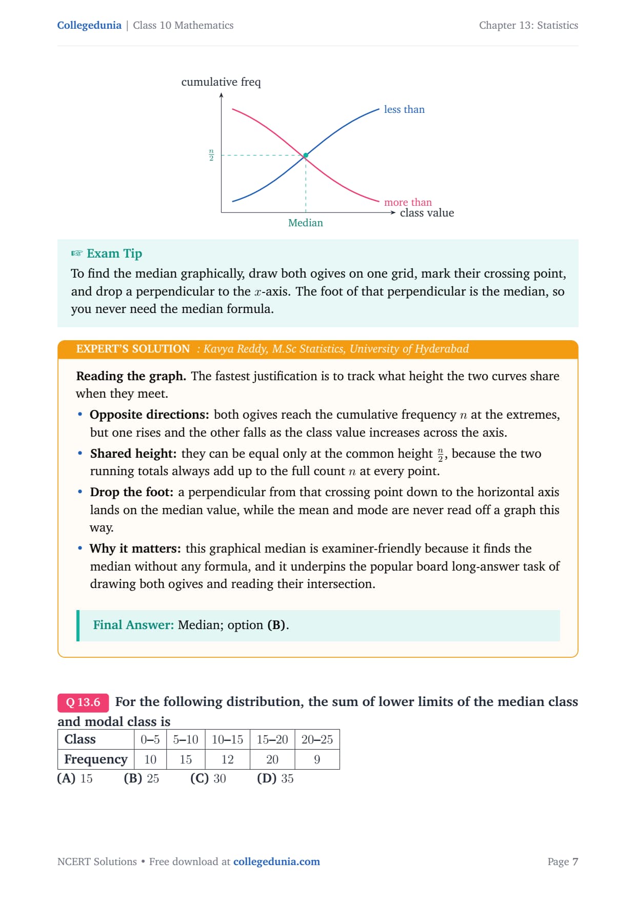
Concept used. An ogive is the graph of a cumulative
frequency distribution. When the less than type ogive and the more than
type ogive are drawn on the same axes, they cross at one point. The
x-coordinate (abscissa) of that crossing point reads off the
median of the data.
Recall what each curve shows: the less than ogive rises with the
running total counted from the bottom; the more than ogive falls
with the running total counted from the top.
At the crossing point both running totals are equal, so each
equals half the total frequency, n2.
The observation value at which exactly n2 items lie
below it is, by definition, the median. So the abscissa of the
intersection is the median.
The abscissa of the intersection of the two ogives is the median; option (B).
KR
Kavya Reddy
M.Sc Statistics, University of Hyderabad
Verified Expert
Reading the graph. The fastest justification is to track what
height the two curves share when they meet.
Opposite directions: both ogives reach the cumulative
frequency n at the extremes, but one rises and the other falls
as the class value increases across the axis.
Shared height: they can be equal only at the common
height n2, because the two running totals always add
up to the full count n at every point.
Drop the foot: a perpendicular from that crossing point
down to the horizontal axis lands on the median value, while the
mean and mode are never read off a graph this way.
Why it matters: this graphical median is
examiner-friendly because it finds the median without any
formula, and it underpins the popular board long-answer task of
drawing both ogives and reading their intersection.
Median; option (B).
Q 13.6
For the following distribution, the sum of lower limits of the median class and modal class is [2pt]
tabular|l|c|c|c|c|c|
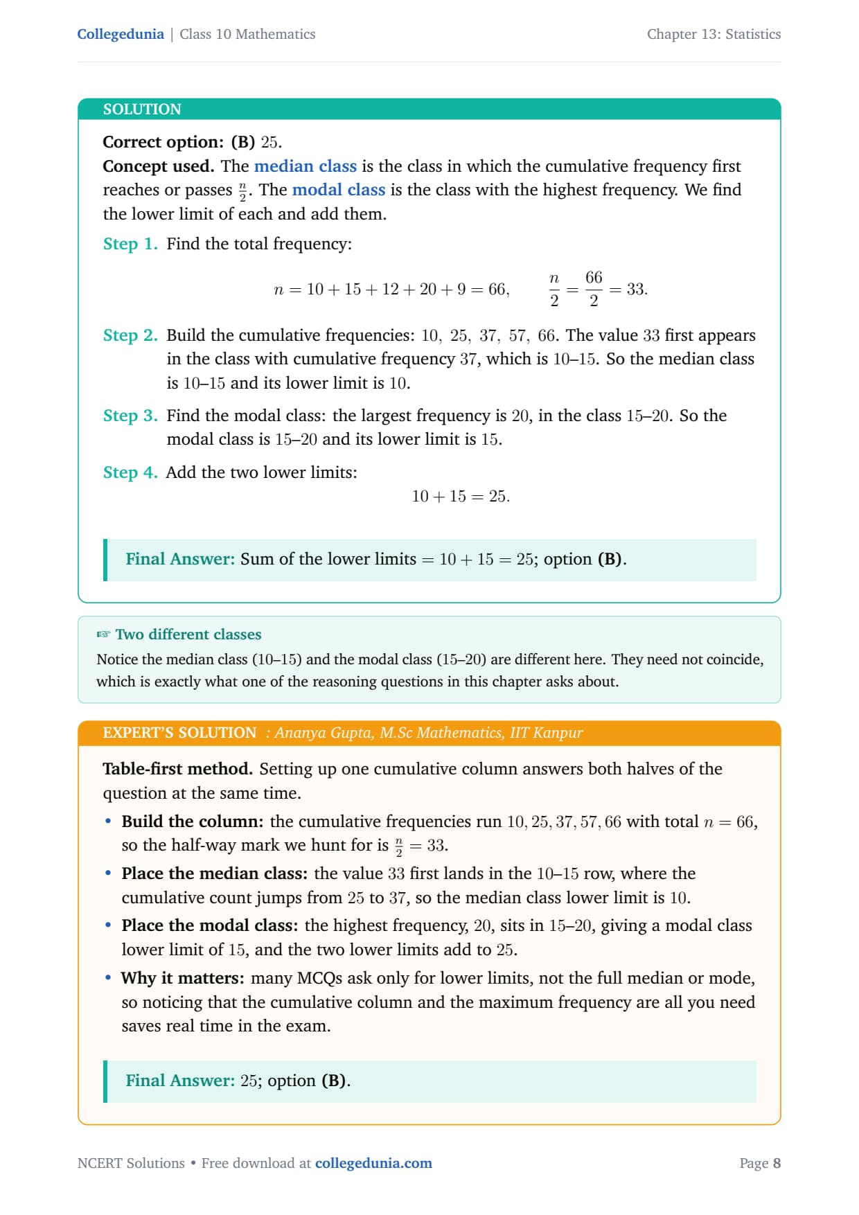
Concept used. The median class is the class in which
the cumulative frequency first reaches or passes n2. The
modal class is the class with the highest frequency. We find
the lower limit of each and add them.
Find the total frequency:
n = 10+15+12+20+9 = 66, n2=662=33.
Build the cumulative frequencies:
10, 25, 37, 57, 66. The value 33 first appears in the
class with cumulative frequency 37, which is 10–15. So the
median class is 10–15 and its lower limit is 10.
Find the modal class: the largest frequency is 20, in the
class 15–20. So the modal class is 15–20 and its lower
limit is 15.
Add the two lower limits:
10 + 15 = 25.
Sum of the lower limits =10+15=25; option (B).
AG
Ananya Gupta
M.Sc Mathematics, IIT Kanpur
Verified Expert
Table-first method. Setting up one cumulative column answers
both halves of the question at the same time.
Build the column: the cumulative frequencies run
10,25,37,57,66 with total n=66, so the half-way mark we hunt
for is n2=33.
Place the median class: the value 33 first lands in
the 10–15 row, where the cumulative count jumps from 25 to
37, so the median class lower limit is 10.
Place the modal class: the highest frequency, 20,
sits in 15–20, giving a modal class lower limit of 15, and
the two lower limits add to 25.
Why it matters: many MCQs ask only for lower limits, not
the full median or mode, so noticing that the cumulative column
and the maximum frequency are all you need saves real time in the
exam.
25; option (B).
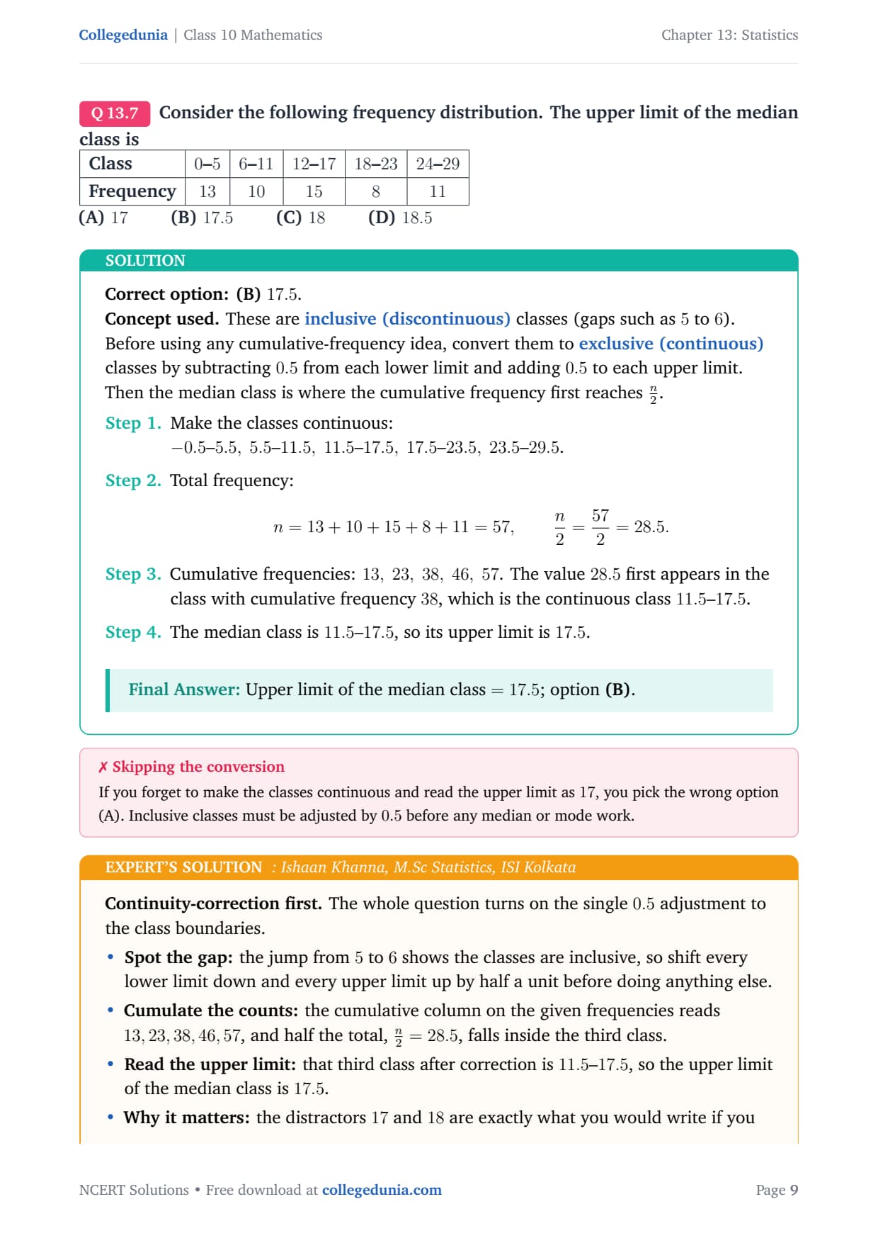
Q 13.7
Consider the following frequency distribution. The upper limit of the median class is [2pt]
tabular|l|c|c|c|c|c|
Concept used. These are inclusive (discontinuous)
classes (gaps such as 5 to 6). Before using any cumulative-frequency
idea, convert them to exclusive (continuous) classes by
subtracting 0.5 from each lower limit and adding 0.5 to each upper
limit. Then the median class is where the cumulative frequency first
reaches n2.
Make the classes continuous:
-0.5–5.5, 5.5–11.5, 11.5–17.5, 17.5–23.5, 23.5–29.5.
Total frequency:
n = 13+10+15+8+11 = 57, n2=572=28.5.
Cumulative frequencies: 13, 23, 38, 46, 57. The value
28.5 first appears in the class with cumulative frequency
38, which is the continuous class 11.5–17.5.
The median class is 11.5–17.5, so its upper limit is
17.5.
Upper limit of the median class =17.5; option (B).
IK
Ishaan Khanna
M.Sc Statistics, ISI Kolkata
Verified Expert
Continuity-correction first. The whole question turns on the
single 0.5 adjustment to the class boundaries.
Spot the gap: the jump from 5 to 6 shows the classes
are inclusive, so shift every lower limit down and every upper
limit up by half a unit before doing anything else.
Cumulate the counts: the cumulative column on the given
frequencies reads 13,23,38,46,57, and half the total,
n2=28.5, falls inside the third class.
Read the upper limit: that third class after correction
is 11.5–17.5, so the upper limit of the median class is
17.5.
Why it matters: the distractors 17 and 18 are
exactly what you would write if you skipped the correction, which
is precisely why examiners slip inclusive classes in to test this
one habit.
17.5; option (B).
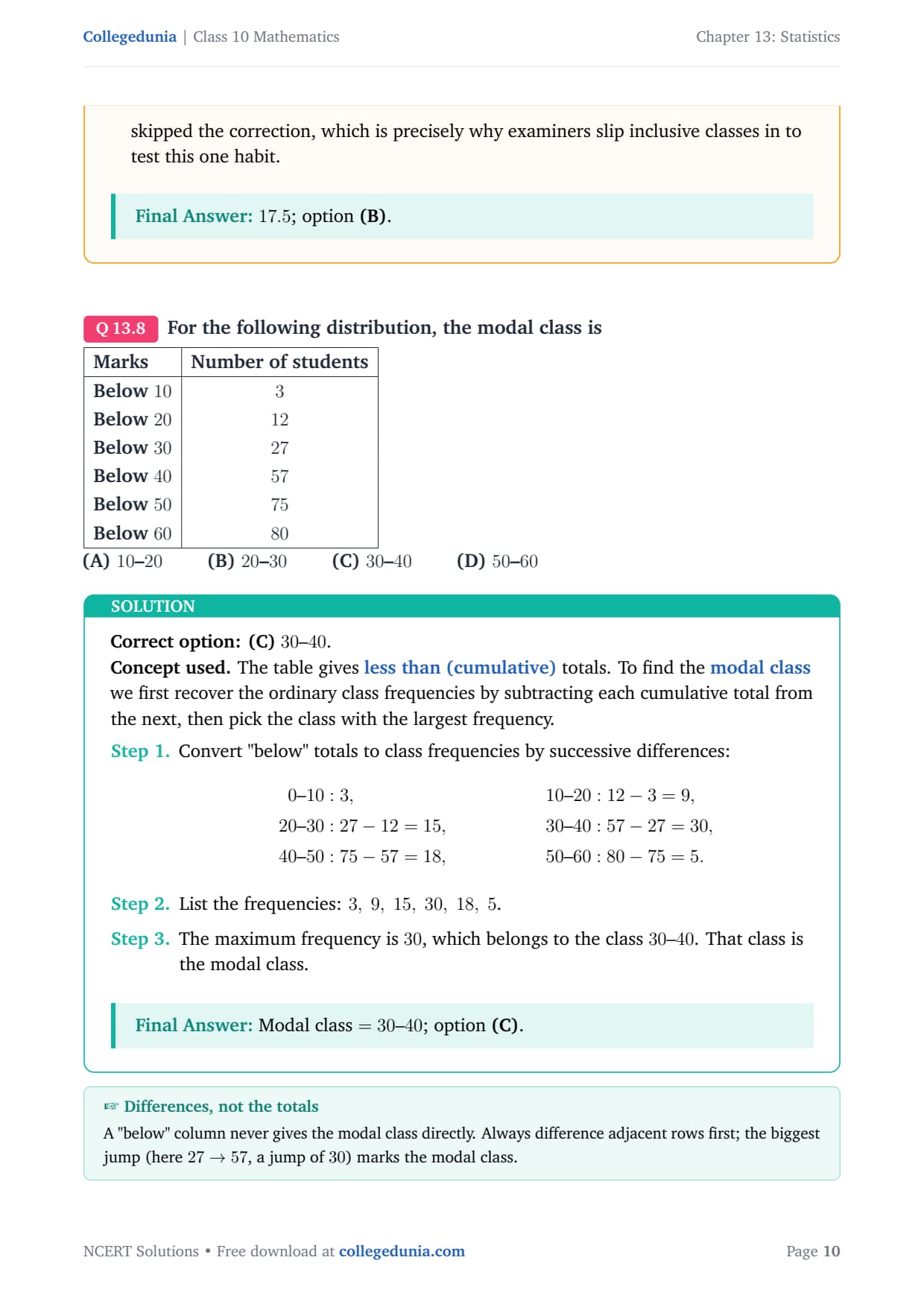
Q 13.8
For the following distribution, the modal class is [2pt]
tabular|l|c|
Marks & Number of students
Below 10 & 3
Below 20 & 12
Below 30 & 27
Below 40 & 57
Below 50 & 75
Below 60 & 80
tabular [2pt]
(A) 10–20 (B) 20–30 (C) 30–40 (D) 50–60
Correct option: (C)30–40.
Concept used. The table gives less than (cumulative)
totals. To find the modal class we first recover the ordinary
class frequencies by subtracting each cumulative total from the next,
then pick the class with the largest frequency.
The maximum frequency is 30, which belongs to the class
30–40. That class is the modal class.
Modal class =30–40; option (C).
MJ
Meera Joshi
M.Sc Mathematics, University of Delhi
Verified Expert
Spotting the biggest jump. The modal class is simply wherever the
cumulative total climbs the fastest.
Difference the totals: subtracting each below row from
the next gives the plain class frequencies 3,9,15,30,18,5,
which is the table you actually need.
Find the steepest rise: the largest single jump is 30,
between Below 30 and Below 40, showing where most students
are packed.
Name the modal class: that jump of 30 is the frequency
of the interval 30–40, so the modal class is 30–40.
Why it matters: reading a cumulative table as if it were
a plain frequency table is a classic slip, but training the eye
to hunt for the biggest jump turns this into a five-second
question.
30–40; option (C).
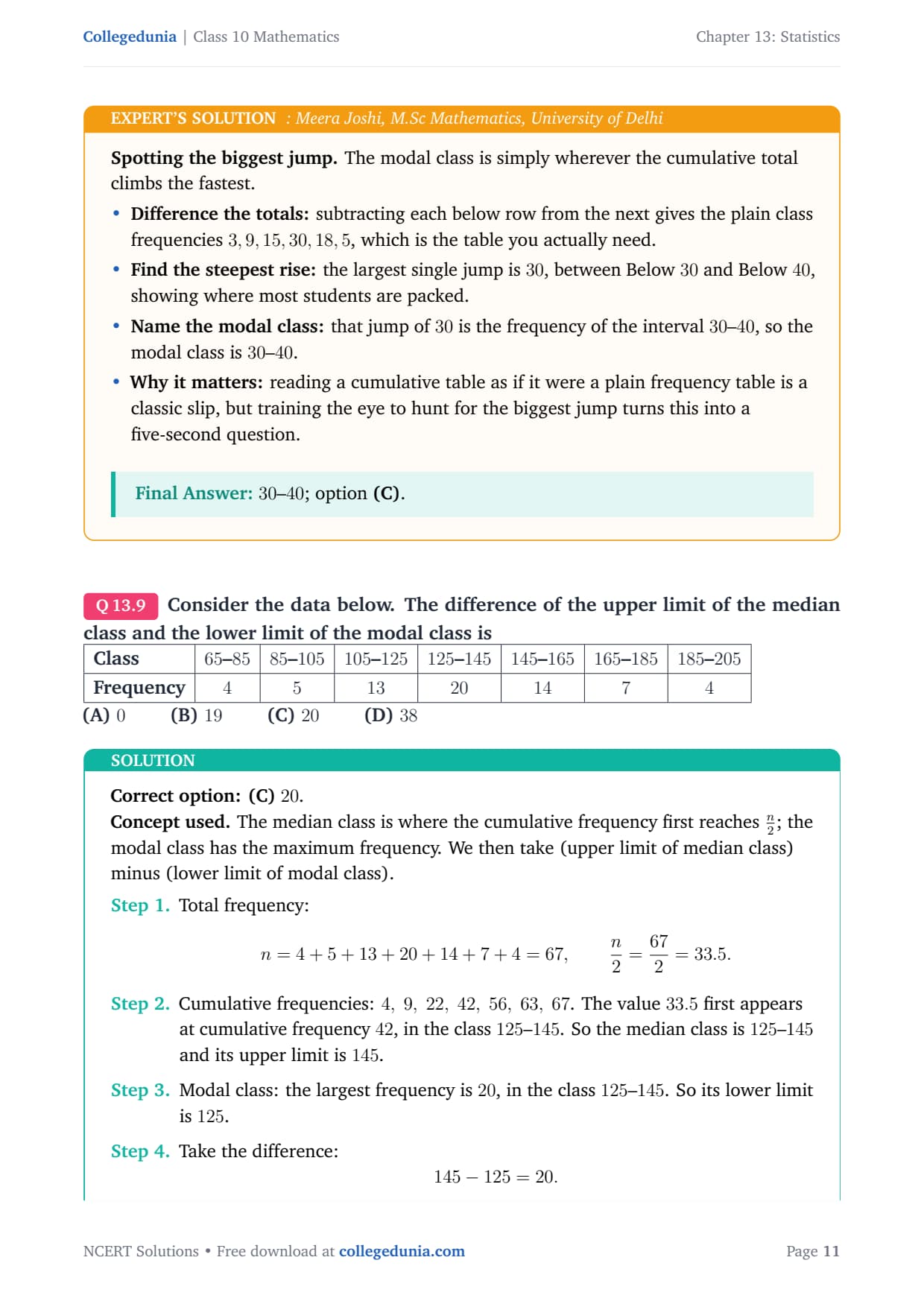
Q 13.9
Consider the data below. The difference of the upper limit of the median class and the lower limit of the modal class is [2pt]
tabular|l|c|c|c|c|c|c|c|
Concept used. The median class is where the cumulative
frequency first reaches n2; the modal class has the maximum
frequency. We then take (upper limit of median class) minus (lower limit
of modal class).
Total frequency:
n = 4+5+13+20+14+7+4 = 67, n2=672=33.5.
Cumulative frequencies:
4, 9, 22, 42, 56, 63, 67. The value 33.5 first appears
at cumulative frequency 42, in the class 125–145. So the
median class is 125–145 and its upper limit is 145.
Modal class: the largest frequency is 20, in the class
125–145. So its lower limit is 125.
Take the difference:
145 - 125 = 20.
Difference =145-125=20; option (C).
AM
Aditya Menon
Ph.D Statistics, IIT Kharagpur
Verified Expert
Width in disguise. When the two classes coincide, the answer is
simply the common class width.
Build the column: the cumulative frequencies are
4,9,22,42,56,63,67, and half the total, n2=33.5,
sits in 125–145, so that is the median class with upper limit
145.
Find the peak: the maximum frequency 20 also belongs
to 125–145, making it the modal class with lower limit 125.
Take the difference: subtracting the lower limit of the
modal class from the upper limit of the median class gives
145-125=20, exactly the width shared by every class.
Why it matters: recognising that this difference
collapses to the class width whenever the two classes agree lets
you check the arithmetic instantly, since each class here spans
20 units.
20; option (C).
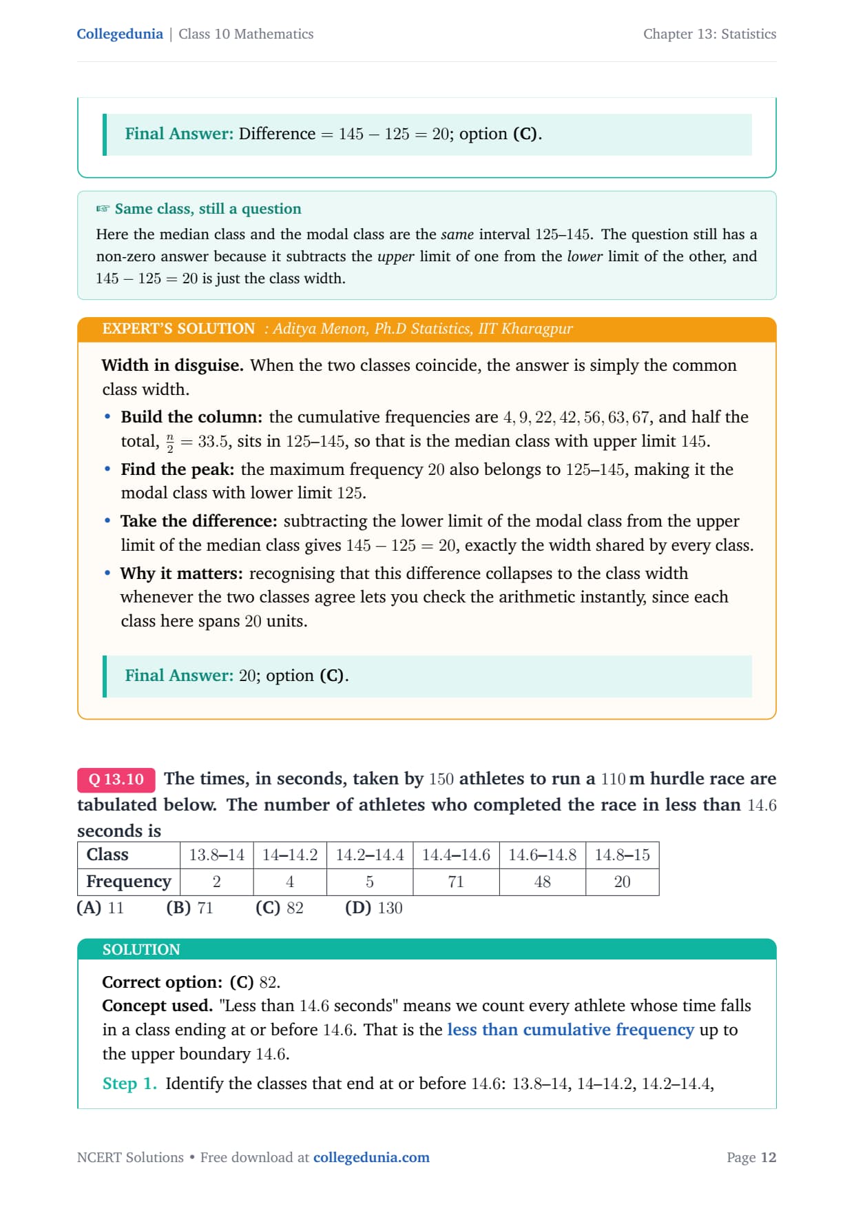
Q 13.10
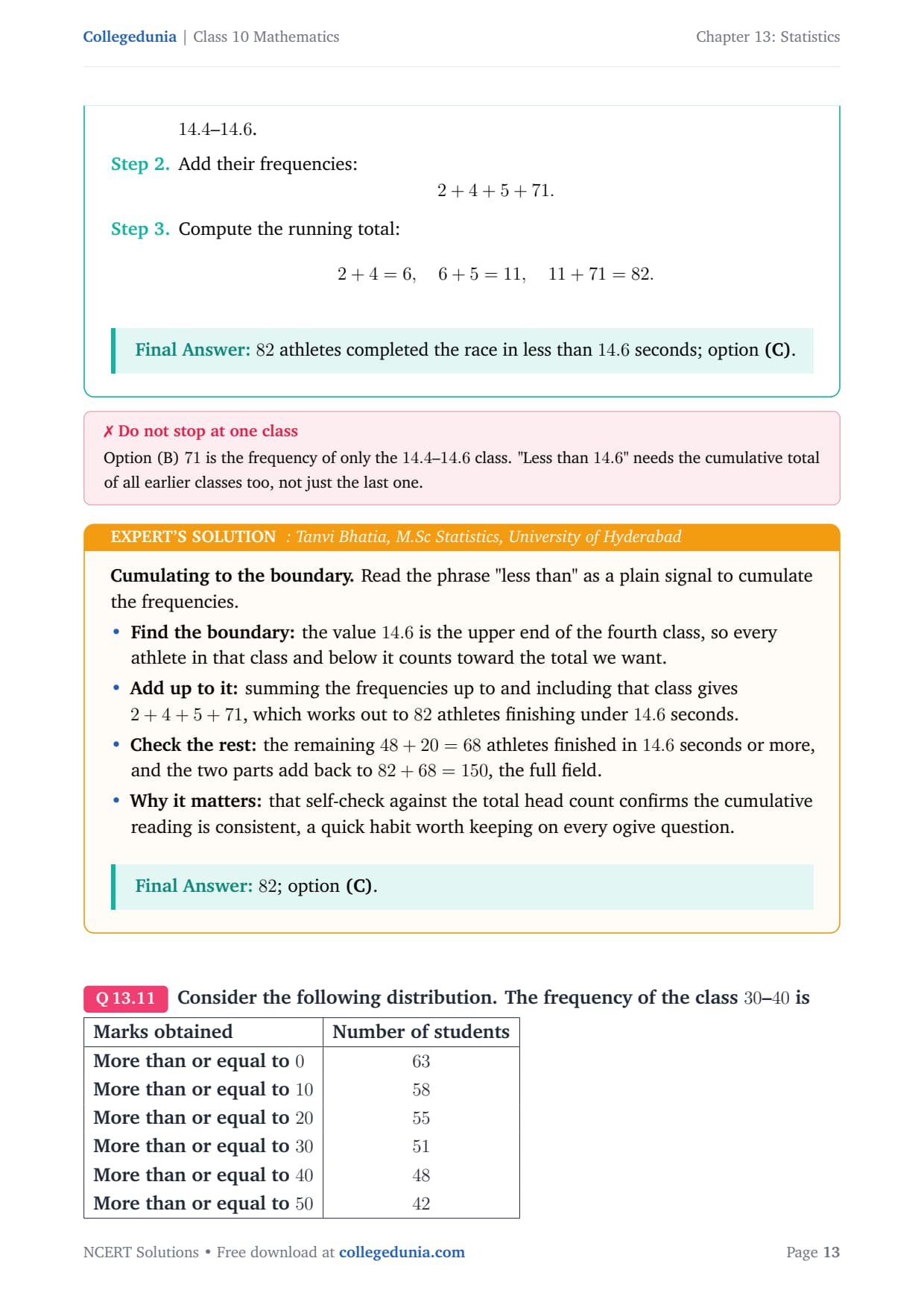
The times, in seconds, taken by 150 athletes to run a 110 m hurdle race are tabulated below. The number of athletes who completed the race in less than 14.6 seconds is [2pt]
tabular|l|c|c|c|c|c|c|
Concept used. "Less than 14.6 seconds" means we count every
athlete whose time falls in a class ending at or before 14.6. That is
the less than cumulative frequency up to the upper boundary
14.6.
Identify the classes that end at or before 14.6:
13.8–14, 14–14.2, 14.2–14.4, 14.4–14.6.
82 athletes completed the race in less than 14.6 seconds; option (C).
TB
Tanvi Bhatia
M.Sc Statistics, University of Hyderabad
Verified Expert
Cumulating to the boundary. Read the phrase "less than" as a
plain signal to cumulate the frequencies.
Find the boundary: the value 14.6 is the upper end of
the fourth class, so every athlete in that class and below it
counts toward the total we want.
Add up to it: summing the frequencies up to and
including that class gives 2+4+5+71, which works out to 82
athletes finishing under 14.6 seconds.
Check the rest: the remaining 48+20=68 athletes
finished in 14.6 seconds or more, and the two parts add back to
82+68=150, the full field.
Why it matters: that self-check against the total head
count confirms the cumulative reading is consistent, a quick
habit worth keeping on every ogive question.
82; option (C).
Q 13.11
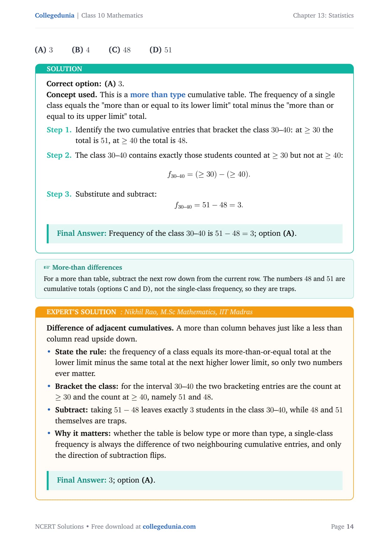
Consider the following distribution. The frequency of the class 30–40 is [2pt]
tabular|l|c|
Marks obtained & Number of students
More than or equal to 0 & 63
More than or equal to 10 & 58
More than or equal to 20 & 55
More than or equal to 30 & 51
More than or equal to 40 & 48
More than or equal to 50 & 42
tabular [2pt]
(A) 3 (B) 4 (C) 48 (D) 51
Correct option: (A)3.
Concept used. This is a more than type cumulative
table. The frequency of a single class equals the "more than or equal to
its lower limit" total minus the "more than or equal to its upper limit"
total.
Identify the two cumulative entries that bracket the class
30–40: at ≥ 30 the total is 51, at ≥ 40 the total
is 48.
The class 30–40 contains exactly those students counted at
≥ 30 but not at ≥ 40:
f30--40 = (≥ 30) - (≥ 40).
Substitute and subtract:
f30--40 = 51 - 48 = 3.
Frequency of the class 30–40 is 51-48=3; option (A).
NR
Nikhil Rao
M.Sc Mathematics, IIT Madras
Verified Expert
Difference of adjacent cumulatives. A more than column behaves
just like a less than column read upside down.
State the rule: the frequency of a class equals its
more-than-or-equal total at the lower limit minus the same total
at the next higher lower limit, so only two numbers ever matter.
Bracket the class: for the interval 30–40 the two
bracketing entries are the count at ≥ 30 and the count at
≥ 40, namely 51 and 48.
Subtract: taking 51-48 leaves exactly 3 students in
the class 30–40, while 48 and 51 themselves are traps.
Why it matters: whether the table is below type or more
than type, a single-class frequency is always the difference of
two neighbouring cumulative entries, and only the direction of
subtraction flips.
3; option (A).
NCERT exemplar Class 12 Mathematics Chapter 13 Statistics
All 4 questions with collapsible Solution and Expert Solution. Tap a button to reveal the working.
II. Short Answer Questions with Reasoning (Exercise 13.2)
Q 13.1
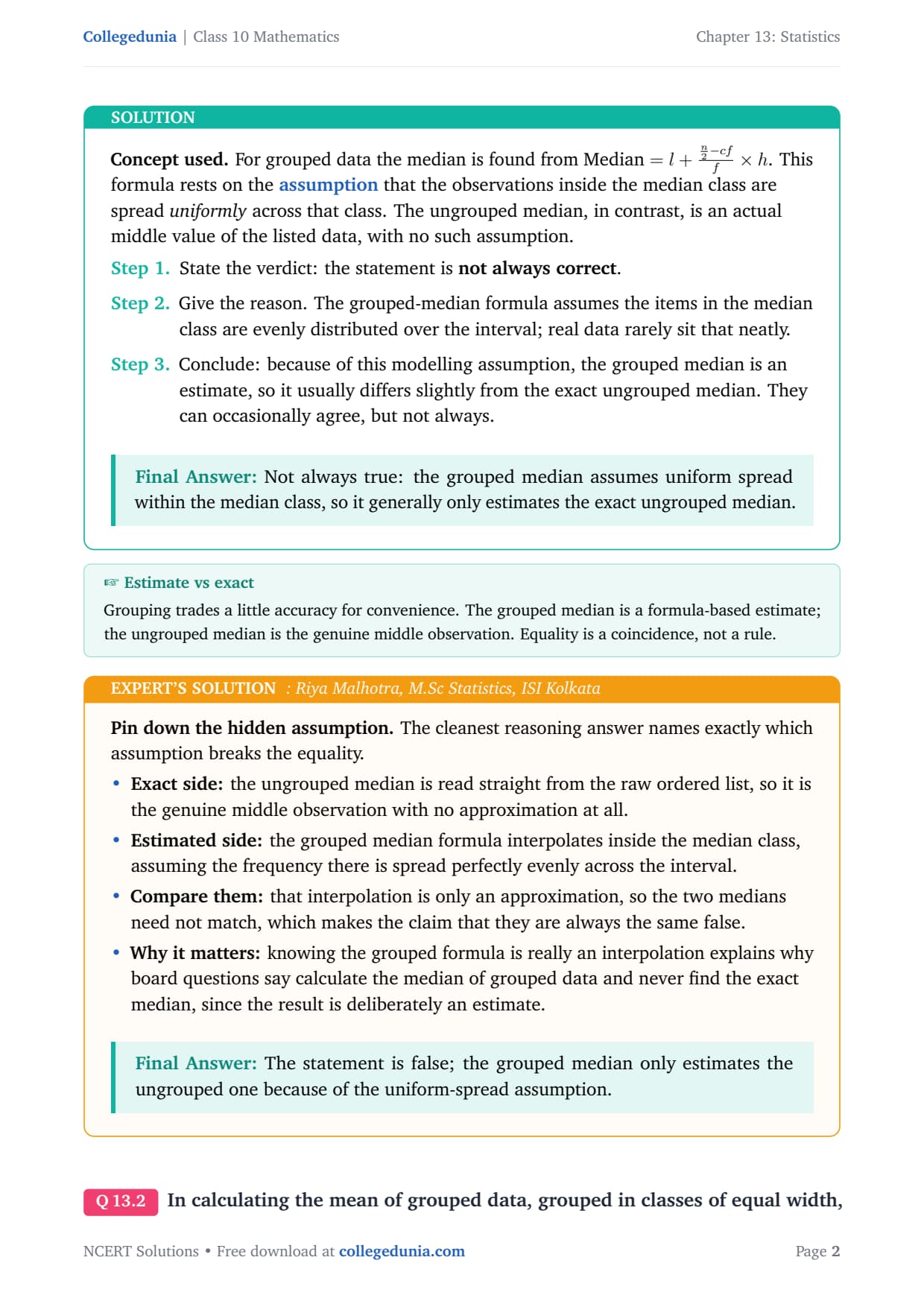
The median of an ungrouped data and the median calculated when the same data is grouped are always the same. Do you think that this is a correct statement? Give reason.
Concept used. For grouped data the median is found from
Median=l+n2-cff× h. This formula rests
on the assumption that the observations inside the median
class are spread uniformly across that class. The ungrouped
median, in contrast, is an actual middle value of the listed data, with
no such assumption.
State the verdict: the statement is not always correct.
Give the reason. The grouped-median formula assumes the items in
the median class are evenly distributed over the interval; real
data rarely sit that neatly.
Conclude: because of this modelling assumption, the grouped
median is an estimate, so it usually differs slightly from the
exact ungrouped median. They can occasionally agree, but not
always.
Not always true: the grouped median assumes uniform spread within the median class, so it generally only estimates the exact ungrouped median.
RM
Riya Malhotra
M.Sc Statistics, ISI Kolkata
Verified Expert
Pin down the hidden assumption. The cleanest reasoning answer
names exactly which assumption breaks the equality.
Exact side: the ungrouped median is read straight from
the raw ordered list, so it is the genuine middle observation
with no approximation at all.
Estimated side: the grouped median formula interpolates
inside the median class, assuming the frequency there is spread
perfectly evenly across the interval.
Compare them: that interpolation is only an
approximation, so the two medians need not match, which makes the
claim that they are always the same false.
Why it matters: knowing the grouped formula is really an
interpolation explains why board questions say calculate the
median of grouped data and never find the exact median, since the
result is deliberately an estimate.
The statement is false; the grouped median only estimates the ungrouped one because of the uniform-spread assumption.
Q 13.2
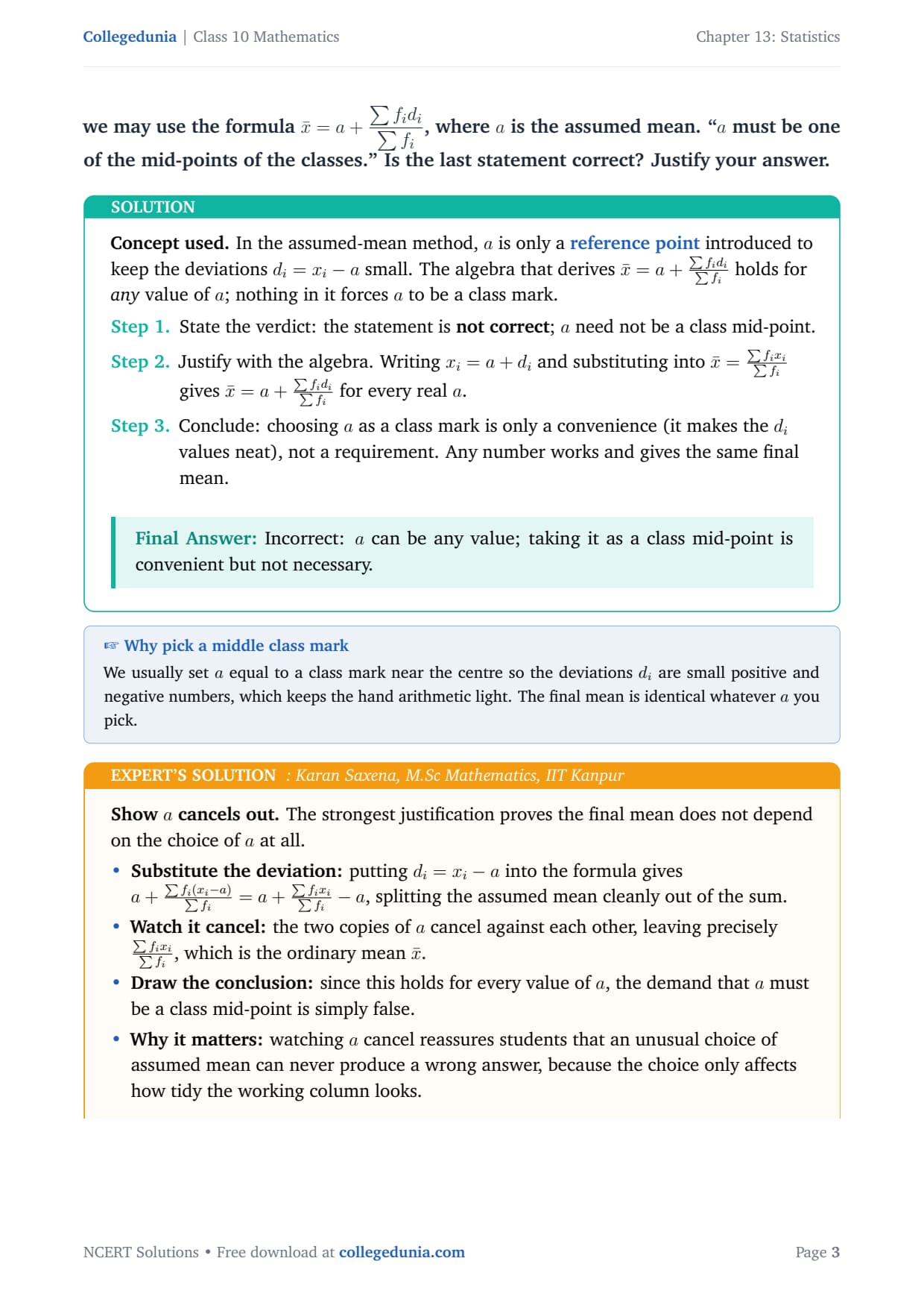
In calculating the mean of grouped data, grouped in classes of equal width, we may use the formula x̄=a+∑ fi di∑ fi, where a is the assumed mean. ``a must be one of the mid-points of the classes.'' Is the last statement correct? Justify your answer.
Concept used. In the assumed-mean method, a is only a
reference point introduced to keep the deviations
di=xi-a small. The algebra that derives
x̄=a+∑ fi di∑ fi holds for any value of
a; nothing in it forces a to be a class mark.
State the verdict: the statement is not correct; a
need not be a class mid-point.
Justify with the algebra. Writing xi=a+di and substituting
into x̄=∑ fi xi∑ fi gives
x̄=a+∑ fi di∑ fi for every real a.
Conclude: choosing a as a class mark is only a convenience
(it makes the di values neat), not a requirement. Any number
works and gives the same final mean.
Incorrect: a can be any value; taking it as a class mid-point is convenient but not necessary.
KS
Karan Saxena
M.Sc Mathematics, IIT Kanpur
Verified Expert
Show a cancels out. The strongest justification proves the
final mean does not depend on the choice of a at all.
Substitute the deviation: putting di=xi-a into the
formula gives
a+∑ fi(xi-a)∑ fi=a+∑ fi xi∑ fi-a,
splitting the assumed mean cleanly out of the sum.
Watch it cancel: the two copies of a cancel against
each other, leaving precisely ∑ fi xi∑ fi,
which is the ordinary mean x̄.
Draw the conclusion: since this holds for every value of
a, the demand that a must be a class mid-point is simply
false.
Why it matters: watching a cancel reassures students
that an unusual choice of assumed mean can never produce a wrong
answer, because the choice only affects how tidy the working
column looks.
The statement is incorrect; the assumed mean a may be any number, not necessarily a class mid-point.
Q 13.3
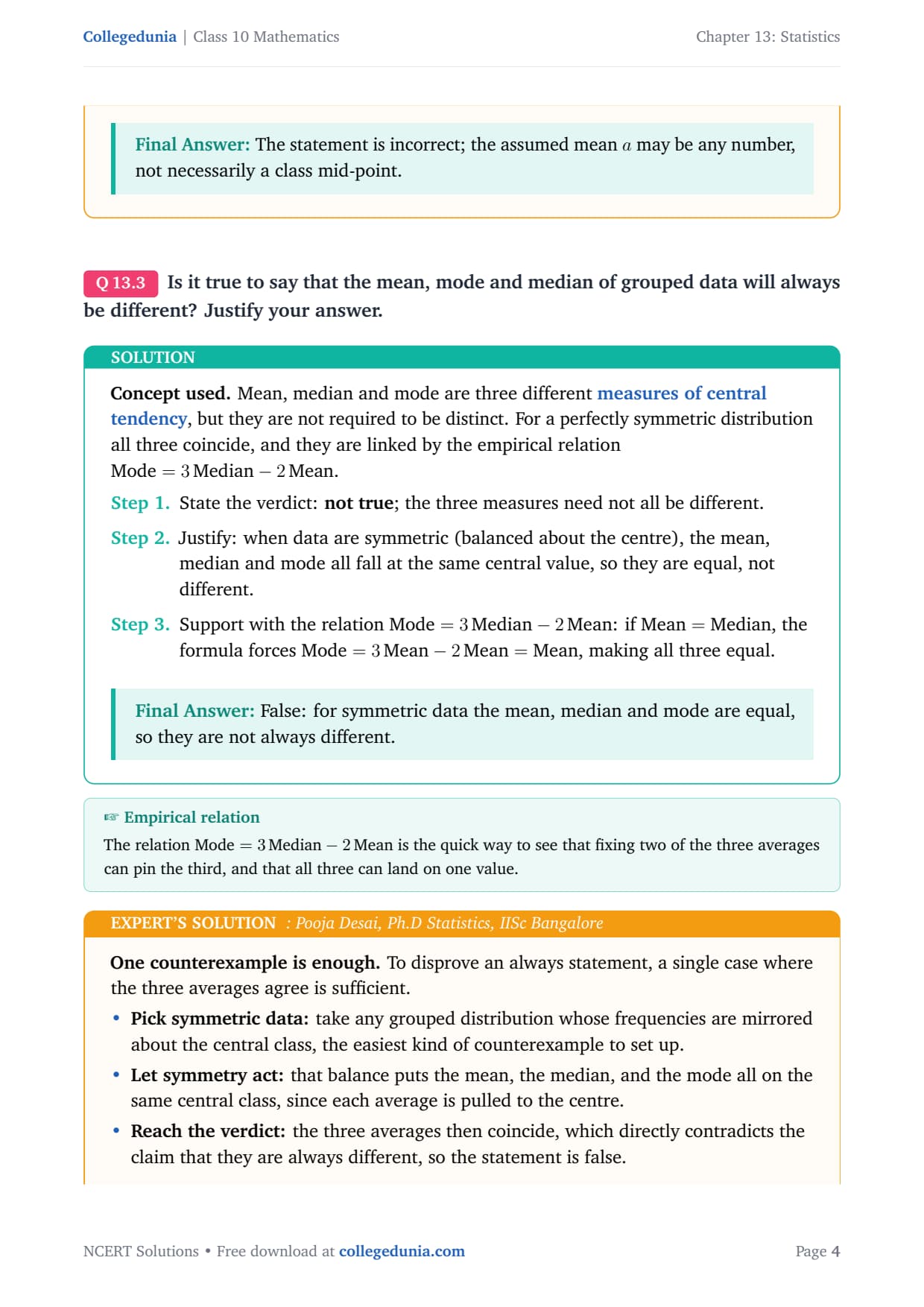
Is it true to say that the mean, mode and median of grouped data will always be different? Justify your answer.
Concept used. Mean, median and mode are three different
measures of central tendency, but they are not required to be
distinct. For a perfectly symmetric distribution all three coincide, and
they are linked by the empirical relation
Mode=3 Median-2 Mean.
State the verdict: not true; the three measures need
not all be different.
Justify: when data are symmetric (balanced about the centre),
the mean, median and mode all fall at the same central value, so
they are equal, not different.
Support with the relation Mode=3 Median-2 Mean:
if Mean=Median, the formula forces
Mode=3 Mean-2 Mean=Mean, making
all three equal.
False: for symmetric data the mean, median and mode are equal, so they are not always different.
PD
Pooja Desai
Ph.D Statistics, IISc Bangalore
Verified Expert
One counterexample is enough. To disprove an always statement,
a single case where the three averages agree is sufficient.
Pick symmetric data: take any grouped distribution whose
frequencies are mirrored about the central class, the easiest
kind of counterexample to set up.
Let symmetry act: that balance puts the mean, the
median, and the mode all on the same central class, since each
average is pulled to the centre.
Reach the verdict: the three averages then coincide,
which directly contradicts the claim that they are always
different, so the statement is false.
Why it matters: the gap between mean, median, and mode
actually measures skewness, and when that gap is zero the data
are symmetric, which is exactly why such always-different claims
break down for balanced data.
The statement is false; symmetric data make the three measures equal.
Q 13.4
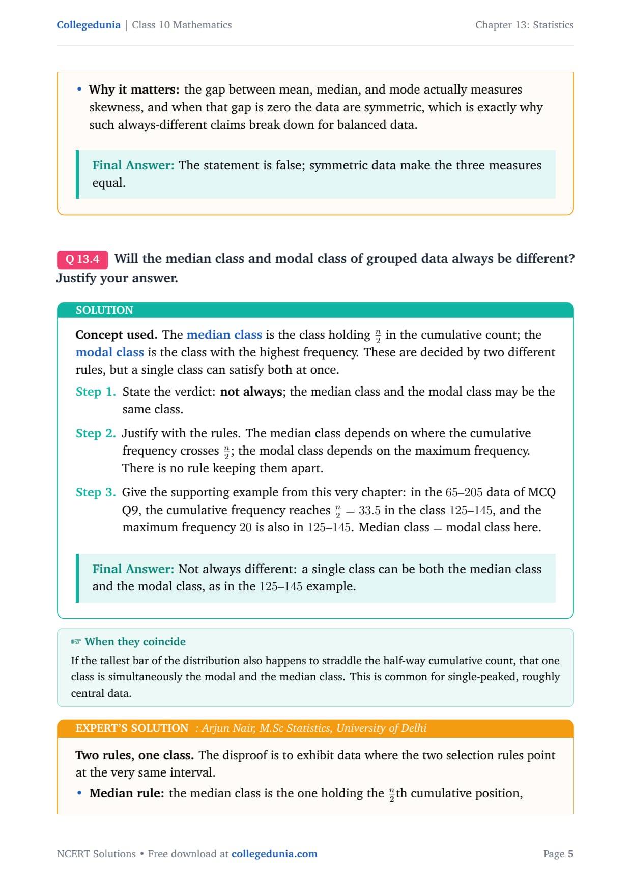
Will the median class and modal class of grouped data always be different? Justify your answer.
Concept used. The median class is the class holding
n2 in the cumulative count; the modal class is the
class with the highest frequency. These are decided by two different
rules, but a single class can satisfy both at once.
State the verdict: not always; the median class and the
modal class may be the same class.
Justify with the rules. The median class depends on where the
cumulative frequency crosses n2; the modal class
depends on the maximum frequency. There is no rule keeping them
apart.
Give the supporting example from this very chapter: in the
65–205 data of MCQ Q9, the cumulative frequency reaches
n2=33.5 in the class 125–145, and the maximum
frequency 20 is also in 125–145. Median class = modal
class here.
Not always different: a single class can be both the median class and the modal class, as in the 125–145 example.
AN
Arjun Nair
M.Sc Statistics, University of Delhi
Verified Expert
Two rules, one class. The disproof is to exhibit data where the
two selection rules point at the very same interval.
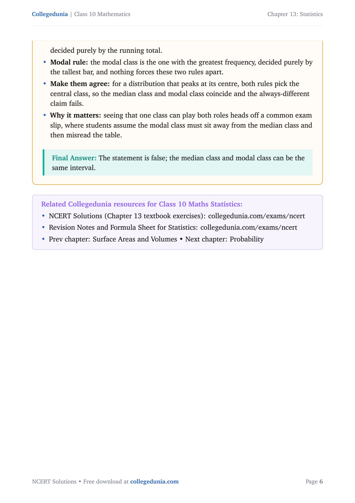
Median rule: the median class is the one holding the
n2th cumulative position, decided purely by the
running total.
Modal rule: the modal class is the one with the greatest
frequency, decided purely by the tallest bar, and nothing forces
these two rules apart.
Make them agree: for a distribution that peaks at its
centre, both rules pick the central class, so the median class
and modal class coincide and the always-different claim fails.
Why it matters: seeing that one class can play both
roles heads off a common exam slip, where students assume the
modal class must sit away from the median class and then misread
the table.
The statement is false; the median class and modal class can be the same interval.
NCERT exemplar Class 12 Mathematics Chapter 13 Statistics
All 18 questions with collapsible Solution and Expert Solution. Tap a button to reveal the working.
III. Short Answer Questions (Exercise 13.3)
Q 13.1
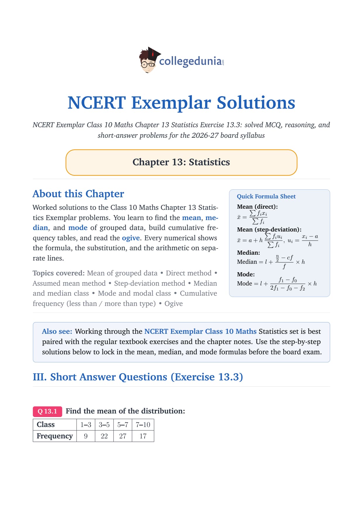
Find the mean of the distribution: [2pt]
tabular|l|c|c|c|c|
Class & 1–3 & 3–5 & 5–7 & 7–10
Frequency & 9 & 22 & 27 & 17
tabular
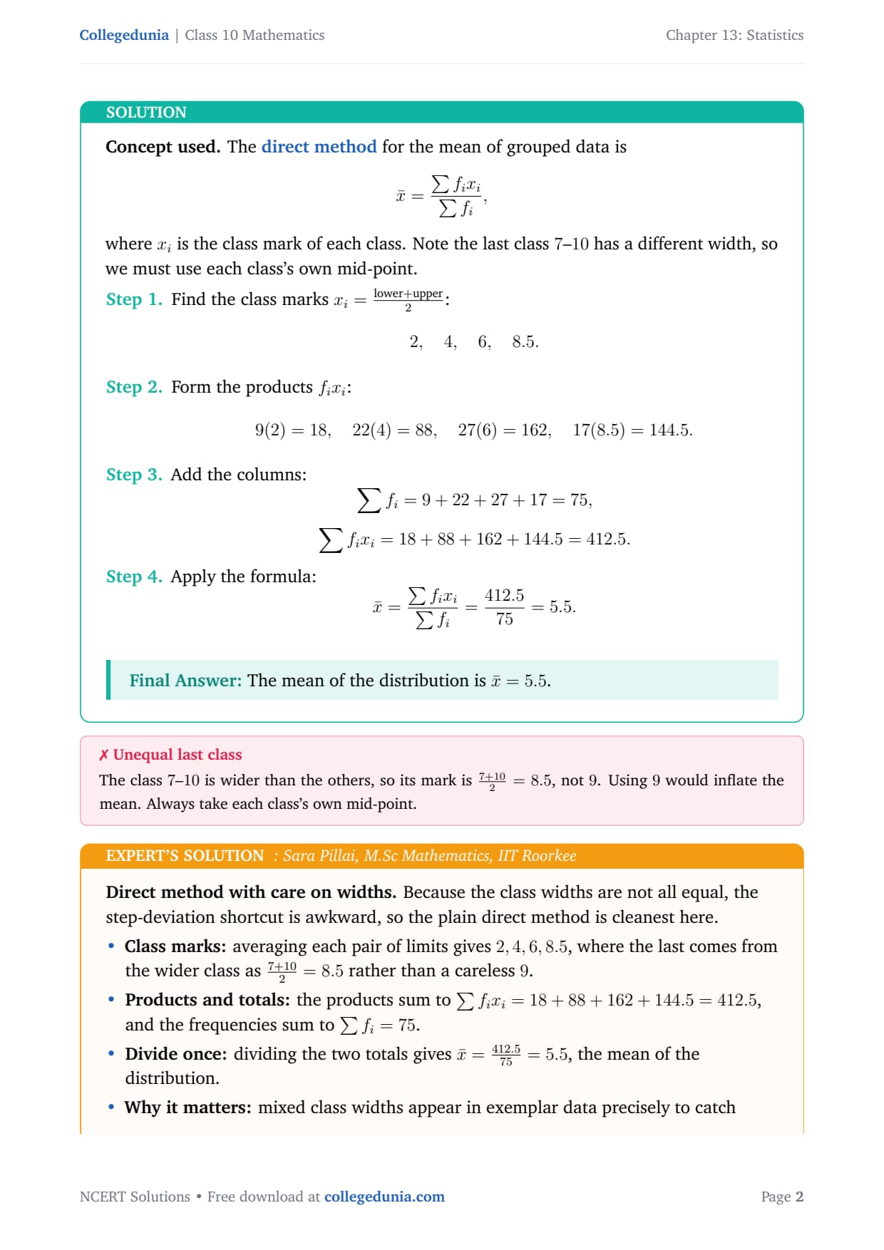
Concept used. The direct method for the mean of
grouped data is
x̄=∑ fi xi∑ fi,
where xi is the class mark of each class. Note the last class
7–10 has a different width, so we must use each class's own
mid-point.
Find the class marks xi=lower+upper2:
2, 4, 6, 8.5.
Form the products fi xi:
9(2)=18, 22(4)=88, 27(6)=162, 17(8.5)=144.5.
Add the columns:
∑ fi = 9+22+27+17 = 75, ∑ fi xi = 18+88+162+144.5 = 412.5.
Apply the formula:
x̄=∑ fi xi∑ fi
=412.575
=5.5.
The mean of the distribution is x̄=5.5.
SP
Sara Pillai
M.Sc Mathematics, IIT Roorkee
Verified Expert
Direct method with care on widths. Because the class widths are
not all equal, the step-deviation shortcut is awkward, so the plain
direct method is cleanest here.
Class marks: averaging each pair of limits gives
2,4,6,8.5, where the last comes from the wider class as
7+102=8.5 rather than a careless 9.
Products and totals: the products sum to
∑ fi xi = 18+88+162+144.5 = 412.5, and the frequencies
sum to ∑ fi = 75.
Divide once: dividing the two totals gives
x̄=412.575=5.5, the mean of the distribution.
Why it matters: mixed class widths appear in exemplar
data precisely to catch students who memorise one class mark and
reuse it, so recomputing xi for every class is the safe habit.
x̄=5.5.
Q 13.2
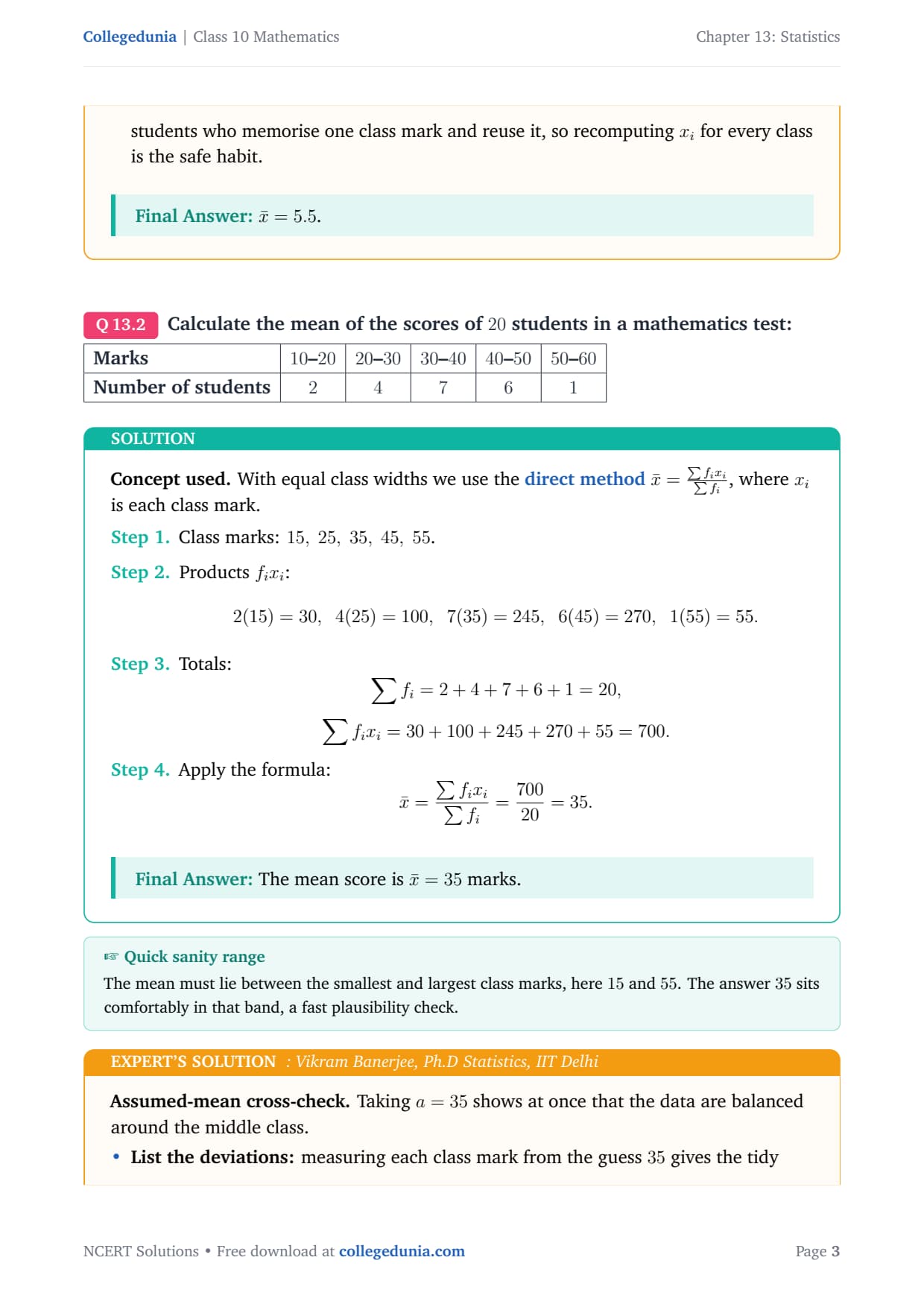
Calculate the mean of the scores of 20 students in a mathematics test: [2pt]
tabular|l|c|c|c|c|c|
Marks & 10–20 & 20–30 & 30–40 & 40–50 & 50–60
Number of students & 2 & 4 & 7 & 6 & 1
tabular
Concept used. With equal class widths we use the direct
methodx̄=∑ fi xi∑ fi, where xi is each
class mark.
Class marks: 15, 25, 35, 45, 55.
Products fi xi:
2(15)=30, 4(25)=100, 7(35)=245, 6(45)=270, 1(55)=55.
Totals:
∑ fi = 2+4+7+6+1 = 20, ∑ fi xi = 30+100+245+270+55 = 700.
Apply the formula:
x̄=∑ fi xi∑ fi
=70020
=35.
The mean score is x̄=35 marks.
VB
Vikram Banerjee
Ph.D Statistics, IIT Delhi
Verified Expert
Assumed-mean cross-check. Taking a=35 shows at once that the
data are balanced around the middle class.
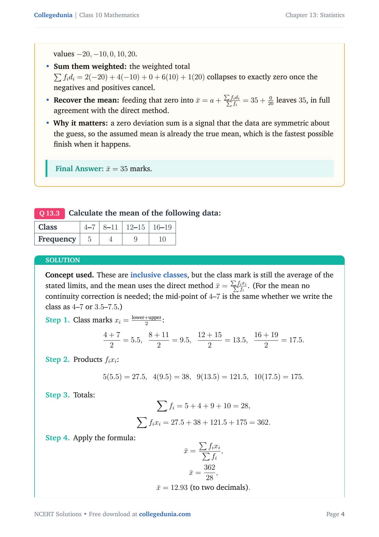
List the deviations: measuring each class mark from the
guess 35 gives the tidy values -20,-10,0,10,20.
Sum them weighted: the weighted total
∑ fi di = 2(-20)+4(-10)+0+6(10)+1(20) collapses to exactly
zero once the negatives and positives cancel.
Recover the mean: feeding that zero into
x̄=a+∑ fi di∑ fi=35+020 leaves
35, in full agreement with the direct method.
Why it matters: a zero deviation sum is a signal that
the data are symmetric about the guess, so the assumed mean is
already the true mean, which is the fastest possible finish when
it happens.
x̄=35 marks.
Q 13.3
Calculate the mean of the following data: [2pt]
tabular|l|c|c|c|c|
Class & 4–7 & 8–11 & 12–15 & 16–19
Frequency & 5 & 4 & 9 & 10
tabular
Concept used. These are inclusive classes, but the
class mark is still the average of the stated limits, and the mean uses
the direct method x̄=∑ fi xi∑ fi. (For the mean
no continuity correction is needed; the mid-point of 4–7 is the same
whether we write the class as 4–7 or 3.5–7.5.)
Class marks xi=lower+upper2:
4+72=5.5, 8+112=9.5,
12+152=13.5, 16+192=17.5.
Products fi xi:
5(5.5)=27.5, 4(9.5)=38, 9(13.5)=121.5, 10(17.5)=175.
Totals:
∑ fi = 5+4+9+10 = 28, ∑ fi xi = 27.5+38+121.5+175 = 362.
Apply the formula:
x̄=∑ fi xi∑ fi, x̄=36228, x̄=12.93 (to two decimals).
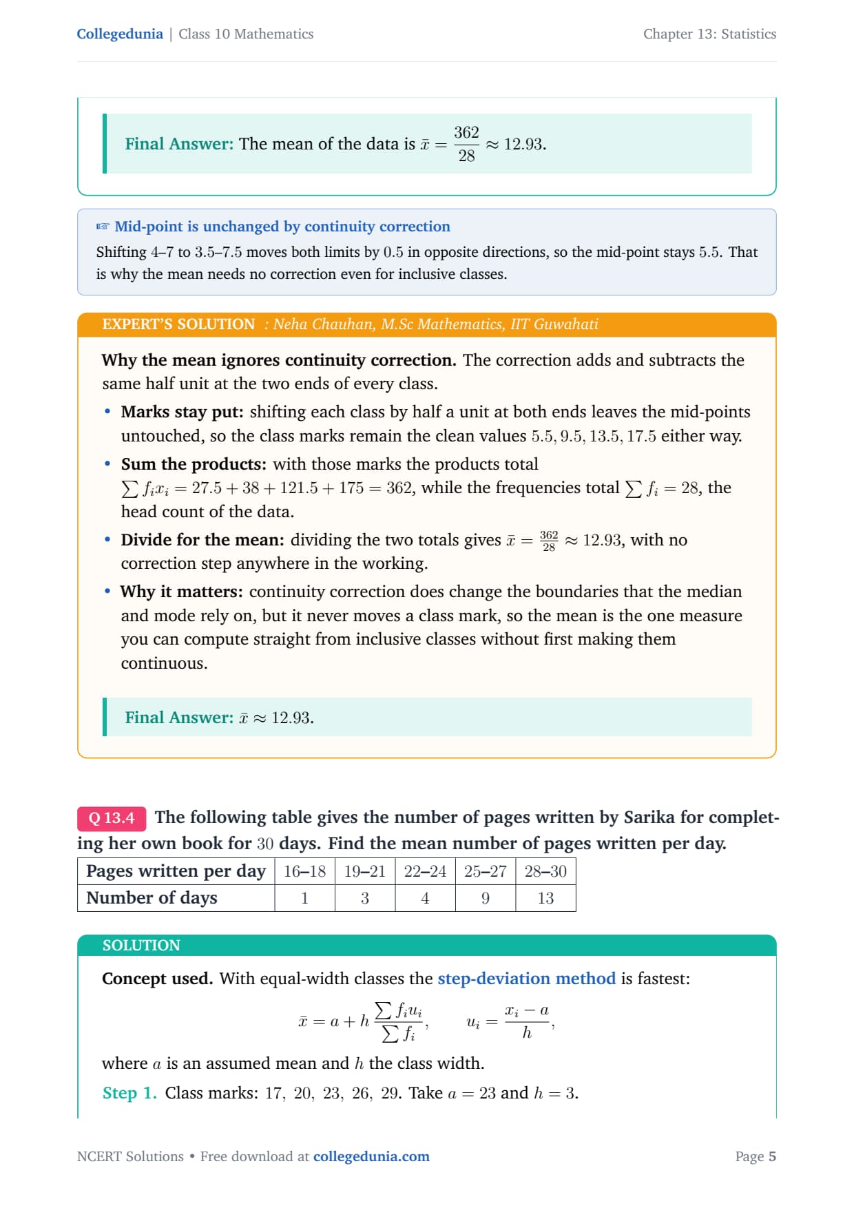
The mean of the data is x̄=36228≈ 12.93.
NC
Neha Chauhan
M.Sc Mathematics, IIT Guwahati
Verified Expert
Why the mean ignores continuity correction. The correction adds
and subtracts the same half unit at the two ends of every class.
Marks stay put: shifting each class by half a unit at
both ends leaves the mid-points untouched, so the class marks
remain the clean values 5.5,9.5,13.5,17.5 either way.
Sum the products: with those marks the products total
∑ fi xi = 27.5+38+121.5+175 = 362, while the frequencies
total ∑ fi = 28, the head count of the data.
Divide for the mean: dividing the two totals gives
x̄=36228≈ 12.93, with no correction step
anywhere in the working.
Why it matters: continuity correction does change the
boundaries that the median and mode rely on, but it never moves a
class mark, so the mean is the one measure you can compute
straight from inclusive classes without first making them
continuous.
x̄≈ 12.93.
Q 13.4
The following table gives the number of pages written by Sarika for completing her own book for 30 days. Find the mean number of pages written per day. [2pt]
tabular|l|c|c|c|c|c|
Pages written per day & 16–18 & 19–21 & 22–24 & 25–27 & 28–30
Number of days & 1 & 3 & 4 & 9 & 13
tabular
Concept used. With equal-width classes the step-deviation
method is fastest:
x̄=a+h∑ fi ui∑ fi, ui=xi-ah,
where a is an assumed mean and h the class width.
Class marks: 17, 20, 23, 26, 29. Take a=23 and
h=3.
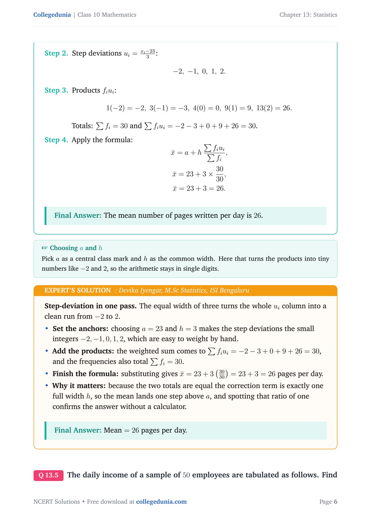
Step deviations ui=xi-233:
-2, -1, 0, 1, 2.
Products fi ui:
1(-2)=-2, 3(-1)=-3, 4(0)=0, 9(1)=9, 13(2)=26.
Totals: ∑ fi = 30 and
∑ fi ui = -2-3+0+9+26 = 30.
Apply the formula:
x̄=a+h∑ fi ui∑ fi, x̄=23+3×3030, x̄=23+3=26.
The mean number of pages written per day is 26.
DI
Devika Iyengar
M.Sc Statistics, ISI Bengaluru
Verified Expert
Step-deviation in one pass. The equal width of three turns the
whole ui column into a clean run from -2 to 2.
Set the anchors: choosing a=23 and h=3 makes the
step deviations the small integers -2,-1,0,1,2, which are easy
to weight by hand.
Add the products: the weighted sum comes to
∑ fi ui = -2-3+0+9+26 = 30, and the frequencies also total
∑ fi = 30.
Finish the formula: substituting gives
x̄=23+3(3030)=23+3=26 pages per day.
Why it matters: because the two totals are equal the
correction term is exactly one full width h, so the mean lands
one step above a, and spotting that ratio of one confirms the
answer without a calculator.
Mean =26 pages per day.
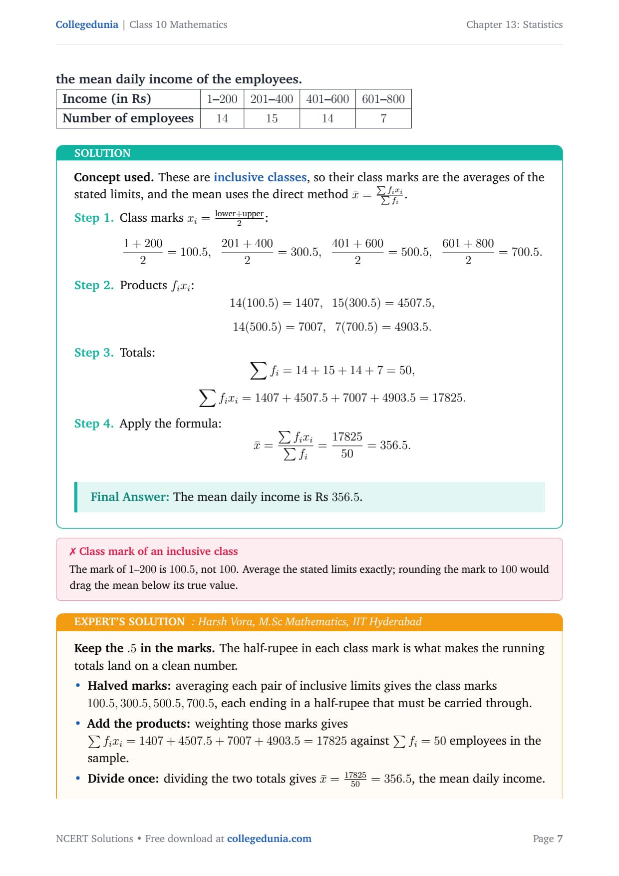
Q 13.5
The daily income of a sample of 50 employees are tabulated as follows. Find the mean daily income of the employees. [2pt]
tabular|l|c|c|c|c|
Income (in Rs) & 1–200 & 201–400 & 401–600 & 601–800
Number of employees & 14 & 15 & 14 & 7
tabular
Concept used. These are inclusive classes, so their
class marks are the averages of the stated limits, and the mean uses the
direct method x̄=∑ fi xi∑ fi.
Class marks xi=lower+upper2:
1+2002=100.5, 201+4002=300.5,
401+6002=500.5, 601+8002=700.5.
Products fi xi:
14(100.5)=1407, 15(300.5)=4507.5, 14(500.5)=7007, 7(700.5)=4903.5.
Totals:
∑ fi = 14+15+14+7 = 50, ∑ fi xi = 1407+4507.5+7007+4903.5 = 17825.
Apply the formula:
x̄=∑ fi xi∑ fi
=1782550
=356.5.
The mean daily income is Rs 356.5.
HV
Harsh Vora
M.Sc Mathematics, IIT Hyderabad
Verified Expert
Keep the .5 in the marks. The half-rupee in each class mark is
what makes the running totals land on a clean number.
Halved marks: averaging each pair of inclusive limits
gives the class marks 100.5,300.5,500.5,700.5, each ending in a
half-rupee that must be carried through.
Add the products: weighting those marks gives
∑ fi xi = 1407+4507.5+7007+4903.5 = 17825 against
∑ fi = 50 employees in the sample.
Divide once: dividing the two totals gives
x̄=1782550=356.5, the mean daily income.
Why it matters: inclusive money brackets like 1–200
are common in real survey data, and carrying the half-rupee
through the whole table prevents a systematic downward bias in the
reported average income.
Mean daily income = Rs 356.5.
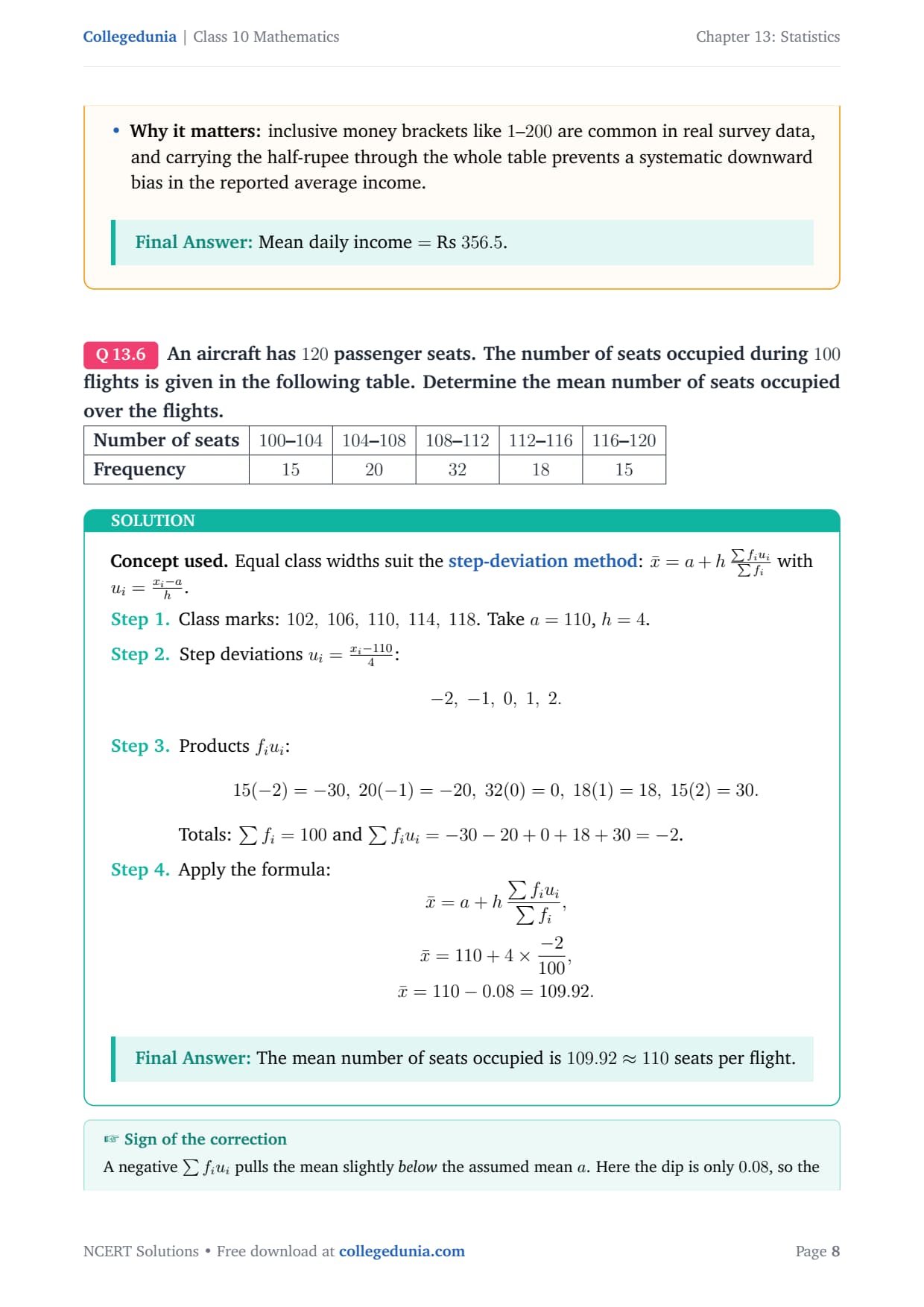
Q 13.6
An aircraft has 120 passenger seats. The number of seats occupied during 100 flights is given in the following table. Determine the mean number of seats occupied over the flights. [2pt]
tabular|l|c|c|c|c|c|
Number of seats & 100–104 & 104–108 & 108–112 & 112–116 & 116–120
Frequency & 15 & 20 & 32 & 18 & 15
tabular
Concept used. Equal class widths suit the step-deviation
method: x̄=a+h∑ fi ui∑ fi with
ui=xi-ah.
Class marks: 102, 106, 110, 114, 118. Take a=110, h=4.
Step deviations ui=xi-1104:
-2, -1, 0, 1, 2.
Products fi ui:
15(-2)=-30, 20(-1)=-20, 32(0)=0, 18(1)=18, 15(2)=30.
Totals: ∑ fi = 100 and
∑ fi ui = -30-20+0+18+30 = -2.
Apply the formula:
x̄=a+h∑ fi ui∑ fi, x̄=110+4×-2100, x̄=110-0.08=109.92.
The mean number of seats occupied is 109.92≈ 110 seats per flight.
LP
Lakshmi Pillai
Ph.D Statistics, IISc Bangalore
Verified Expert
Small correction, large a. The assumed mean does the heavy
lifting while the step column only nudges it a little.
Set the anchors: taking a=110 and h=4 gives the
usual step deviations -2,-1,0,1,2, centred on the busiest band.
Add the products: the weighted total is only
∑ fi ui = -2 against a head count of ∑ fi = 100, so
the correction will be small.
Finish the formula: substituting gives
x̄=110+4(-2100)=110-0.08=109.92 seats.
Why it matters: when data are nearly symmetric about the
central class the step sum is tiny and the mean settles very close
to a, which is a handy estimate-first check before you trust the
final decimal.
Mean =109.92 seats.
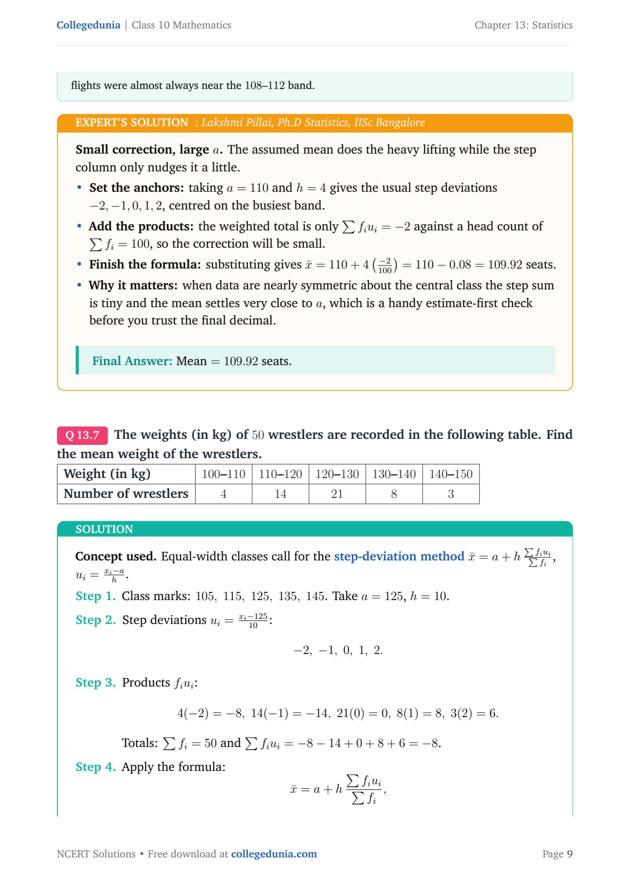
Q 13.7
The weights (in kg) of 50 wrestlers are recorded in the following table. Find the mean weight of the wrestlers. [2pt]
tabular|l|c|c|c|c|c|
Weight (in kg) & 100–110 & 110–120 & 120–130 & 130–140 & 140–150
Number of wrestlers & 4 & 14 & 21 & 8 & 3
tabular
Concept used. Equal-width classes call for the
step-deviation methodx̄=a+h∑ fi ui∑ fi, ui=xi-ah.
Class marks: 105, 115, 125, 135, 145. Take a=125, h=10.
Step deviations ui=xi-12510:
-2, -1, 0, 1, 2.
Products fi ui:
4(-2)=-8, 14(-1)=-14, 21(0)=0, 8(1)=8, 3(2)=6.
Totals: ∑ fi = 50 and
∑ fi ui = -8-14+0+8+6 = -8.
Apply the formula:
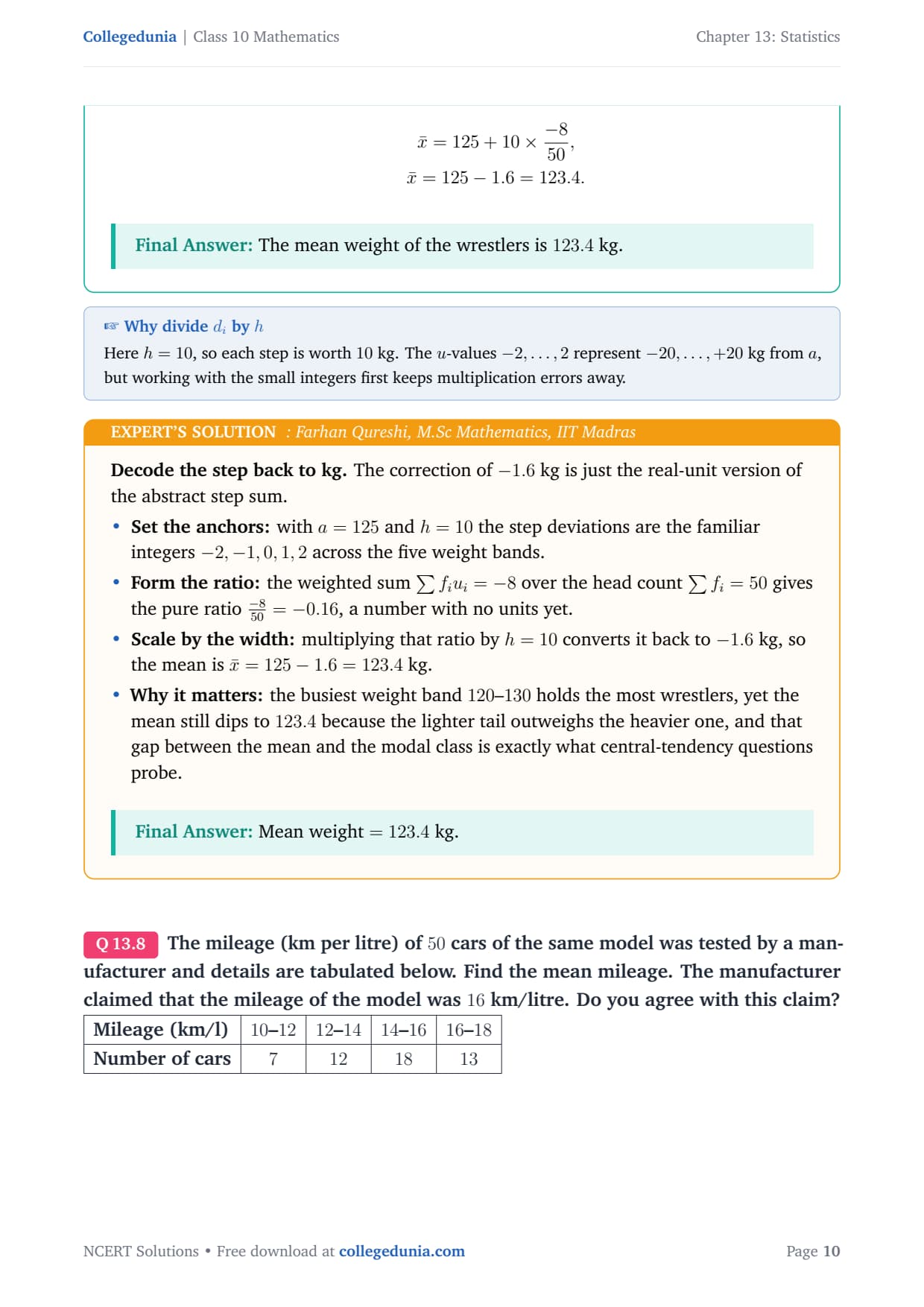
x̄=a+h∑ fi ui∑ fi, x̄=125+10×-850, x̄=125-1.6=123.4.
The mean weight of the wrestlers is 123.4 kg.
FQ
Farhan Qureshi
M.Sc Mathematics, IIT Madras
Verified Expert
Decode the step back to kg. The correction of -1.6 kg is just
the real-unit version of the abstract step sum.
Set the anchors: with a=125 and h=10 the step
deviations are the familiar integers -2,-1,0,1,2 across the five
weight bands.
Form the ratio: the weighted sum ∑ fi ui = -8 over
the head count ∑ fi = 50 gives the pure ratio
-850=-0.16, a number with no units yet.
Scale by the width: multiplying that ratio by h=10
converts it back to -1.6 kg, so the mean is
x̄=125-1.6=123.4 kg.
Why it matters: the busiest weight band 120–130
holds the most wrestlers, yet the mean still dips to 123.4
because the lighter tail outweighs the heavier one, and that gap
between the mean and the modal class is exactly what
central-tendency questions probe.
Mean weight =123.4 kg.
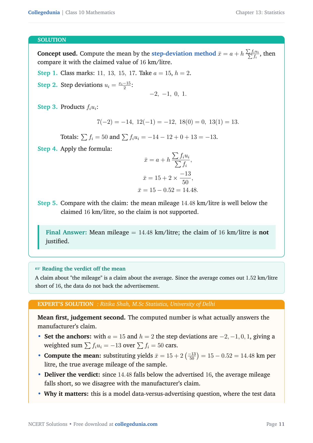
Q 13.8
The mileage (km per litre) of 50 cars of the same model was tested by a manufacturer and details are tabulated below. Find the mean mileage. The manufacturer claimed that the mileage of the model was 16 km/litre. Do you agree with this claim? [2pt]
tabular|l|c|c|c|c|
Concept used. Compute the mean by the step-deviation
methodx̄=a+h∑ fi ui∑ fi, then compare it
with the claimed value of 16 km/litre.
Class marks: 11, 13, 15, 17. Take a=15, h=2.
Step deviations ui=xi-152:
-2, -1, 0, 1.
Products fi ui:
7(-2)=-14, 12(-1)=-12, 18(0)=0, 13(1)=13.
Totals: ∑ fi = 50 and
∑ fi ui = -14-12+0+13 = -13.
Apply the formula:
x̄=a+h∑ fi ui∑ fi, x̄=15+2×-1350, x̄=15-0.52=14.48.
Compare with the claim: the mean mileage 14.48 km/litre is
well below the claimed 16 km/litre, so the claim is not
supported.
Mean mileage =14.48 km/litre; the claim of 16 km/litre is not justified.
RS
Ritika Shah
M.Sc Statistics, University of Delhi
Verified Expert
Mean first, judgement second. The computed number is what
actually answers the manufacturer's claim.
Set the anchors: with a=15 and h=2 the step
deviations are -2,-1,0,1, giving a weighted sum
∑ fi ui=-13 over ∑ fi=50 cars.
Compute the mean: substituting yields
x̄=15+2(-1350)=15-0.52=14.48 km per
litre, the true average mileage of the sample.
Deliver the verdict: since 14.48 falls below the
advertised 16, the average mileage falls short, so we disagree
with the manufacturer's claim.
Why it matters: this is a model data-versus-advertising
question, where the test data give a defensible average and any
marketing figure above it must be challenged, so always anchor the
verdict to the computed mean rather than the single best class.
x̄=14.48 km/litre; the 16 km/litre claim is not agreed.
Q 13.9
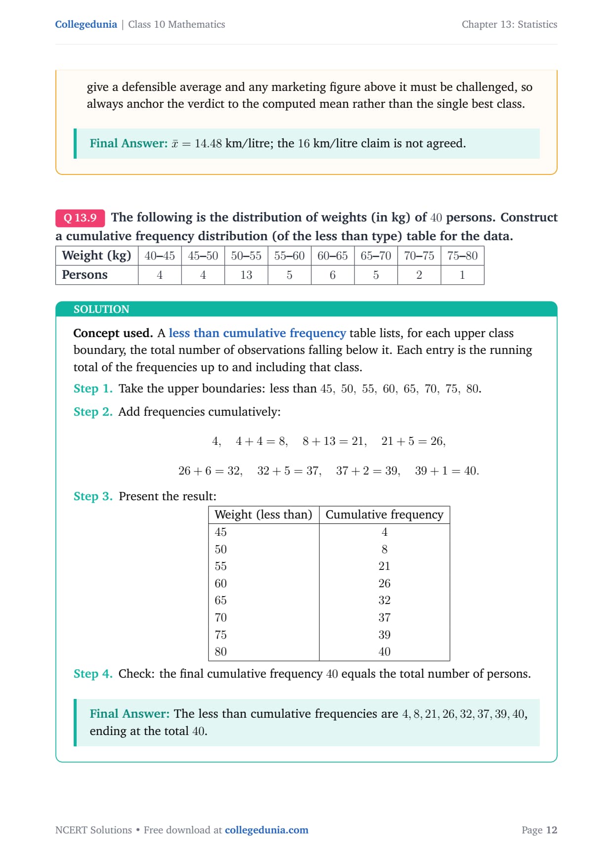
The following is the distribution of weights (in kg) of 40 persons. Construct a cumulative frequency distribution (of the less than type) table for the data. [2pt]
tabular|l|c|c|c|c|c|c|c|c|
Concept used. A less than cumulative frequency table
lists, for each upper class boundary, the total number of observations
falling below it. Each entry is the running total of the frequencies up
to and including that class.
Take the upper boundaries: less than 45, 50, 55, 60, 65,
70, 75, 80.
Check: the final cumulative frequency 40 equals the total
number of persons.
The less than cumulative frequencies are 4,8,21,26,32,37,39,40, ending at the total 40.
OA
Ovais Ahmed
M.Sc Statistics, ISI Kolkata
Verified Expert
Running-total discipline. Build the column from the top and
never re-sum it from scratch at each row.
Start the chain: take the first frequency, 4, as the
opening cumulative total, since nothing lies below the lowest
class.
Add one at a time: fold each next frequency into the
running total to produce 4,8,21,26,32,37,39,40 in a single
downward pass.
Check the end: the eighth total is 40, equal to the
number of persons, which confirms the column is internally
consistent.
Why it matters: this less than column is exactly the set
of plotting points for a less than ogive, with the upper boundary
on the horizontal axis and the cumulative count on the vertical
axis, which several board long-answer problems then ask you to
graph.
Cumulative frequencies 4,8,21,26,32,37,39,40.
Q 13.10
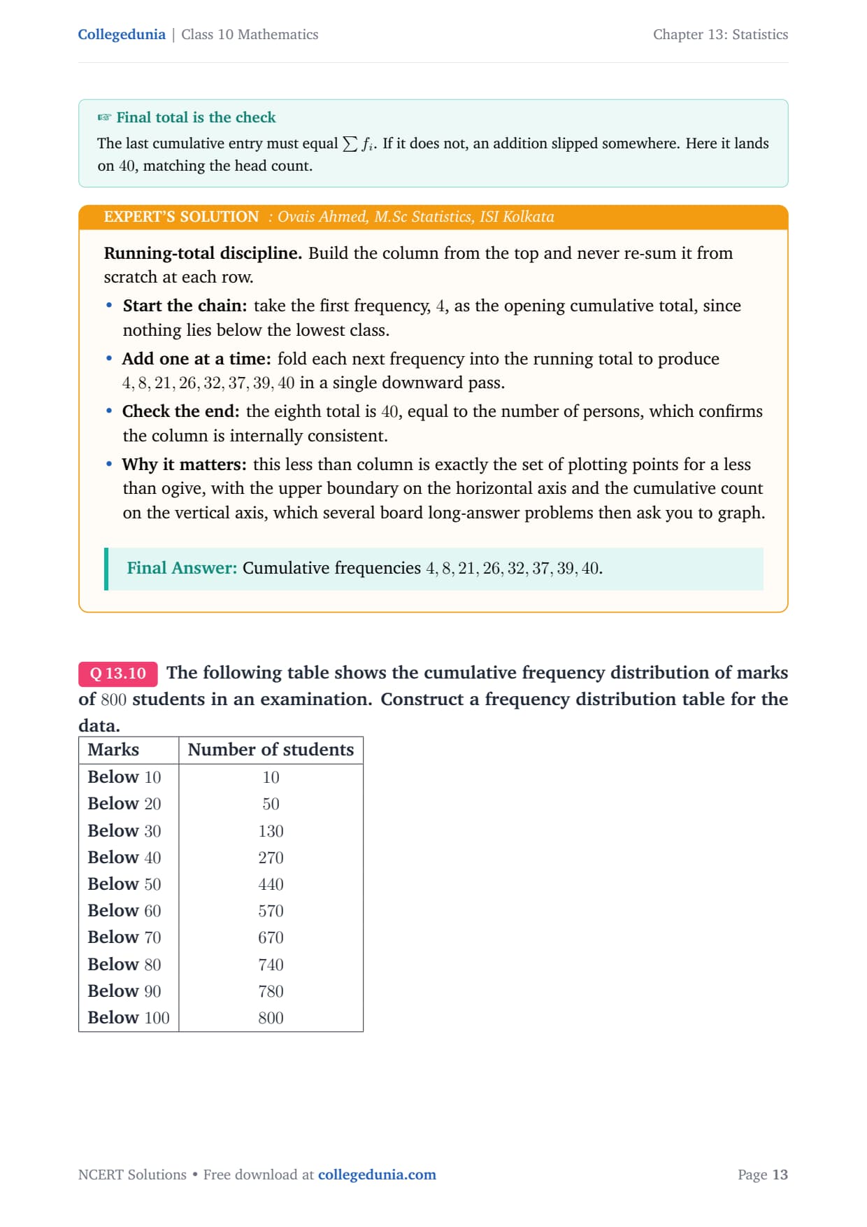
The following table shows the cumulative frequency distribution of marks of 800 students in an examination. Construct a frequency distribution table for the data. [2pt]
tabular|l|c|
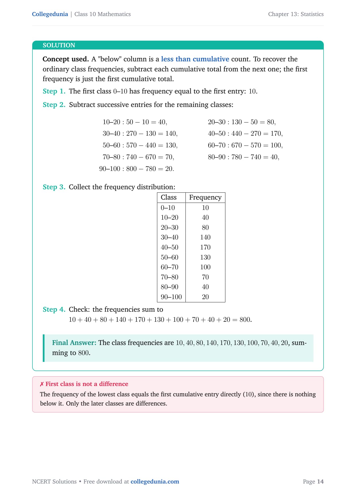
Concept used. A "below" column is a less than
cumulative count. To recover the ordinary class frequencies, subtract
each cumulative total from the next one; the first frequency is just the
first cumulative total.
The first class 0–10 has frequency equal to the first entry:
10.
Check: the frequencies sum to
10+40+80+140+170+130+100+70+40+20 = 800.
The class frequencies are 10,40,80,140,170,130,100,70,40,20, summing to 800.
BR
Bhavna Reddy
M.Sc Mathematics, IIT Bombay
Verified Expert
Differencing a cumulative column. A below column adds one class
at a time as the marks rise, so reversing it means taking the gap between
each pair of neighbouring totals.
First row is special: no marks lie below 10, so the
first cumulative total is also the first class frequency, making
the frequency of 0–10 simply 10.
Difference the rest: for every later class the frequency
is the current below total minus the previous one, so 30–40
gives 270-130=140 and 40–50 gives 440-270=170.
Read down the column: working steadily downward produces
the full frequency list 10,40,80,140,170,130,100,70,40,20 in
ascending class order.
Verify the total: adding them gives
10+40+80+140+170+130+100+70+40+20=800, the number of students,
so no row was mis-subtracted.
Why it matters: the peak frequency 170 sits in the
class 40–50, marking it as the modal class, and recovering
this plain frequency column is the necessary first step before
any mode, median, or histogram work on cumulative data.
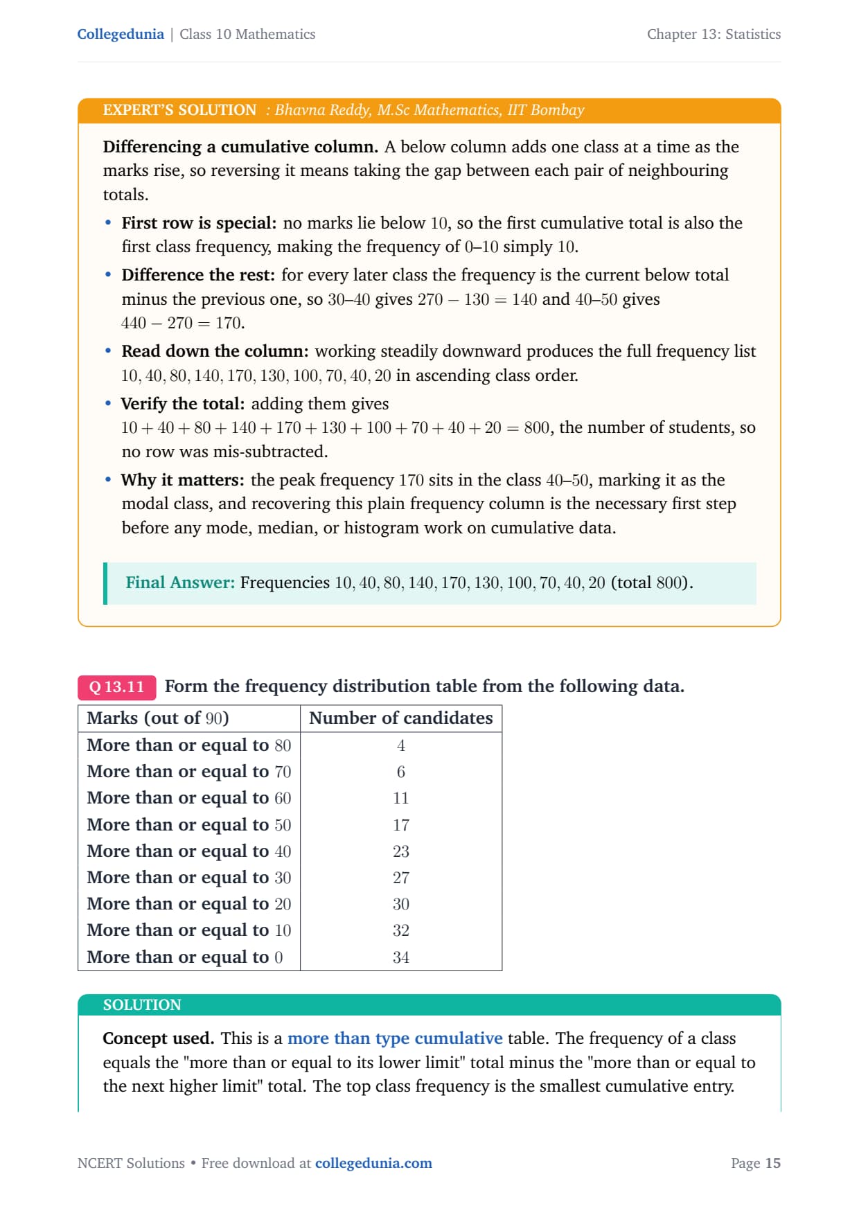
Form the frequency distribution table from the following data. [2pt]
tabular|l|c|
Marks (out of 90) & Number of candidates
More than or equal to 80 & 4
More than or equal to 70 & 6
More than or equal to 60 & 11
More than or equal to 50 & 17
More than or equal to 40 & 23
More than or equal to 30 & 27
More than or equal to 20 & 30
More than or equal to 10 & 32
More than or equal to 0 & 34
tabular
Concept used. This is a more than type cumulative
table. The frequency of a class equals the "more than or equal to its
lower limit" total minus the "more than or equal to the next higher
limit" total. The top class frequency is the smallest cumulative entry.
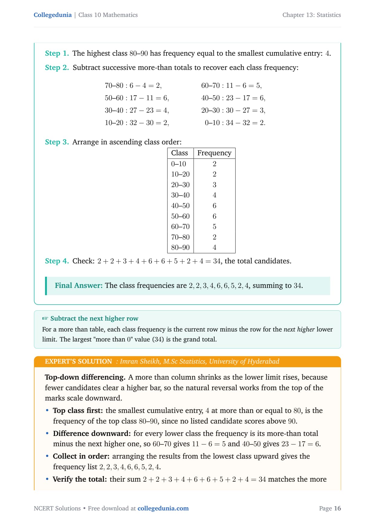
The highest class 80–90 has frequency equal to the smallest
cumulative entry: 4.
Check: 2+2+3+4+6+6+5+2+4 = 34, the total candidates.
The class frequencies are 2,2,3,4,6,6,5,2,4, summing to 34.
IS
Imran Sheikh
M.Sc Statistics, University of Hyderabad
Verified Expert
Top-down differencing. A more than column shrinks as the lower
limit rises, because fewer candidates clear a higher bar, so the natural
reversal works from the top of the marks scale downward.
Top class first: the smallest cumulative entry, 4 at
more than or equal to 80, is the frequency of the top class
80–90, since no listed candidate scores above 90.
Difference downward: for every lower class the frequency
is its more-than total minus the next higher one, so 60–70
gives 11-6=5 and 40–50 gives 23-17=6.
Collect in order: arranging the results from the lowest
class upward gives the frequency list 2,2,3,4,6,6,5,2,4.
Verify the total: their sum
2+2+3+4+6+6+5+2+4=34 matches the more than or equal to 0
entry exactly, so the differencing is consistent.
Why it matters: a more than table is the data behind a
more than ogive that falls from left to right, and recovering the
plain frequencies lets you cross-check that curve against its less
than partner, whose intersection pins the median.
Frequencies 2,2,3,4,6,6,5,2,4 (total 34).
Q 13.12
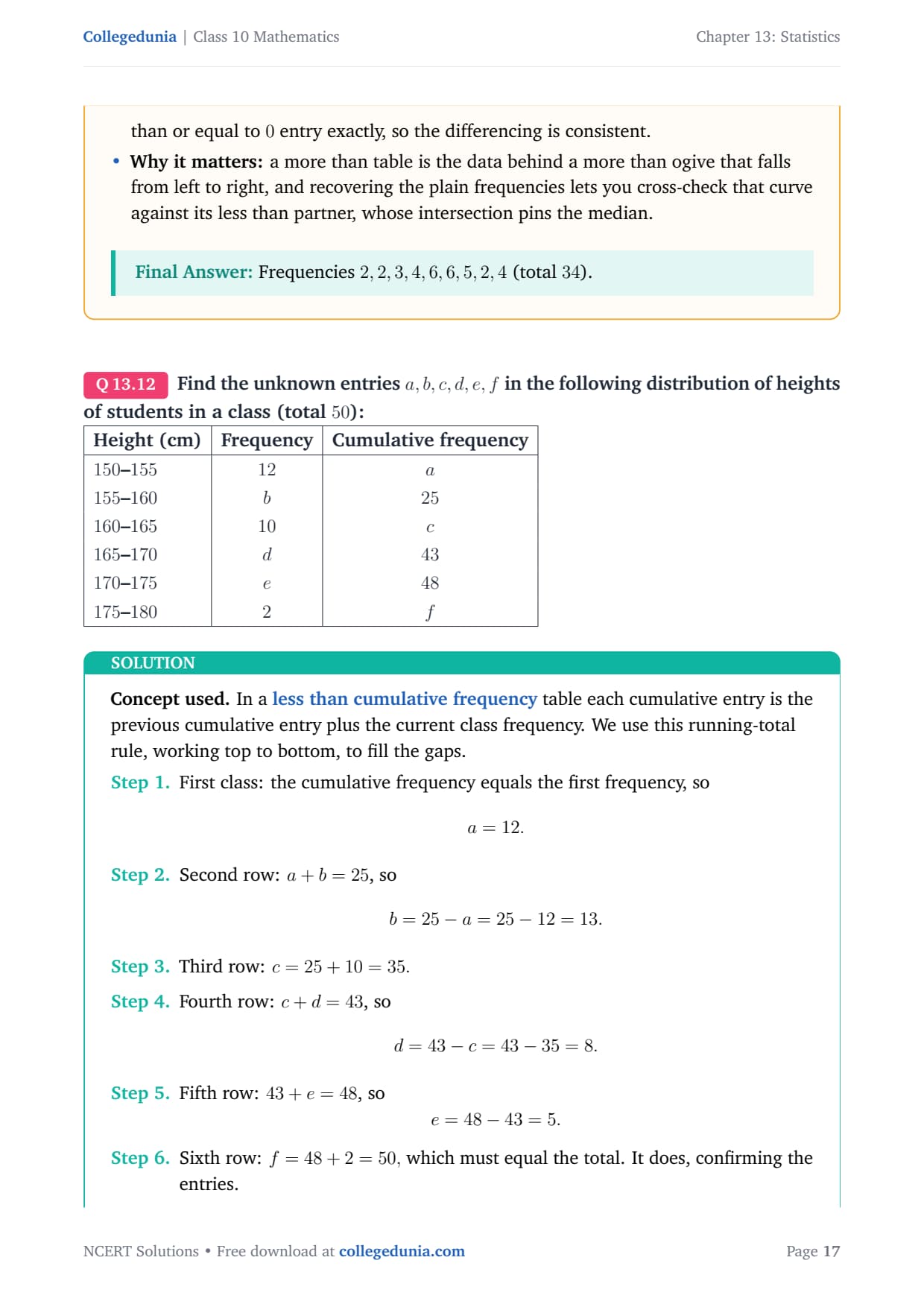
Find the unknown entries a,b,c,d,e,f in the following distribution of heights of students in a class (total 50): [2pt]
tabular|l|c|c|
Height (cm) & Frequency & Cumulative frequency 150–155 & 12 & a 155–160 & b & 25 160–165 & 10 & c 165–170 & d & 43 170–175 & e & 48 175–180 & 2 & f
tabular
Concept used. In a less than cumulative frequency
table each cumulative entry is the previous cumulative entry plus the
current class frequency. We use this running-total rule, working top to
bottom, to fill the gaps.
First class: the cumulative frequency equals the first
frequency, so
a = 12.
Second row: a+b=25, so
b = 25 - a = 25 - 12 = 13.
Third row: c = 25 + 10 = 35.
Fourth row: c + d = 43, so
d = 43 - c = 43 - 35 = 8.
Fifth row: 43 + e = 48, so
e = 48 - 43 = 5.
Sixth row: f = 48 + 2 = 50, which must equal the total. It
does, confirming the entries.
a=12, b=13, c=35, d=8, e=5, f=50.
GD
Gauri Deshpande
M.Sc Mathematics, IIT Madras
Verified Expert
Walk the running total. Each unknown is just one add or one
subtract away from its neighbour in the table.
Open the chain: the entry a is the first cumulative
value, which equals the first frequency, so a=12 straight away.
Fill the gaps: reading the cumulative gaps gives
b=25-12=13, then c=25+10=35, then d=43-35=8, then
e=48-43=5, one neighbour at a time.
Close the chain: the last cumulative value
f=48+2=50 equals the stated total, confirming every earlier
unknown was found correctly.
Why it matters: mixing the two columns is the common
trap, since the frequency column is built from differences while
the cumulative column is built from running sums, so keeping the
two rules apart makes find-the-unknowns routine.
a=12, b=13, c=35, d=8, e=5, f=50.
Q 13.13
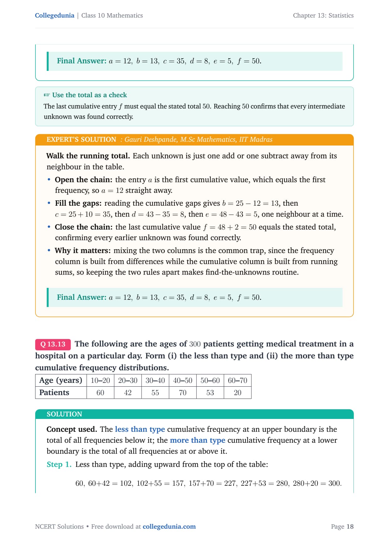
The following are the ages of 300 patients getting medical treatment in a hospital on a particular day. Form (i) the less than type and (ii) the more than type cumulative frequency distributions. [2pt]
tabular|l|c|c|c|c|c|c|
Concept used. The less than type cumulative frequency
at an upper boundary is the total of all frequencies below it; the
more than type cumulative frequency at a lower boundary is the
total of all frequencies at or above it.
Less than type, adding upward from the top of the table:
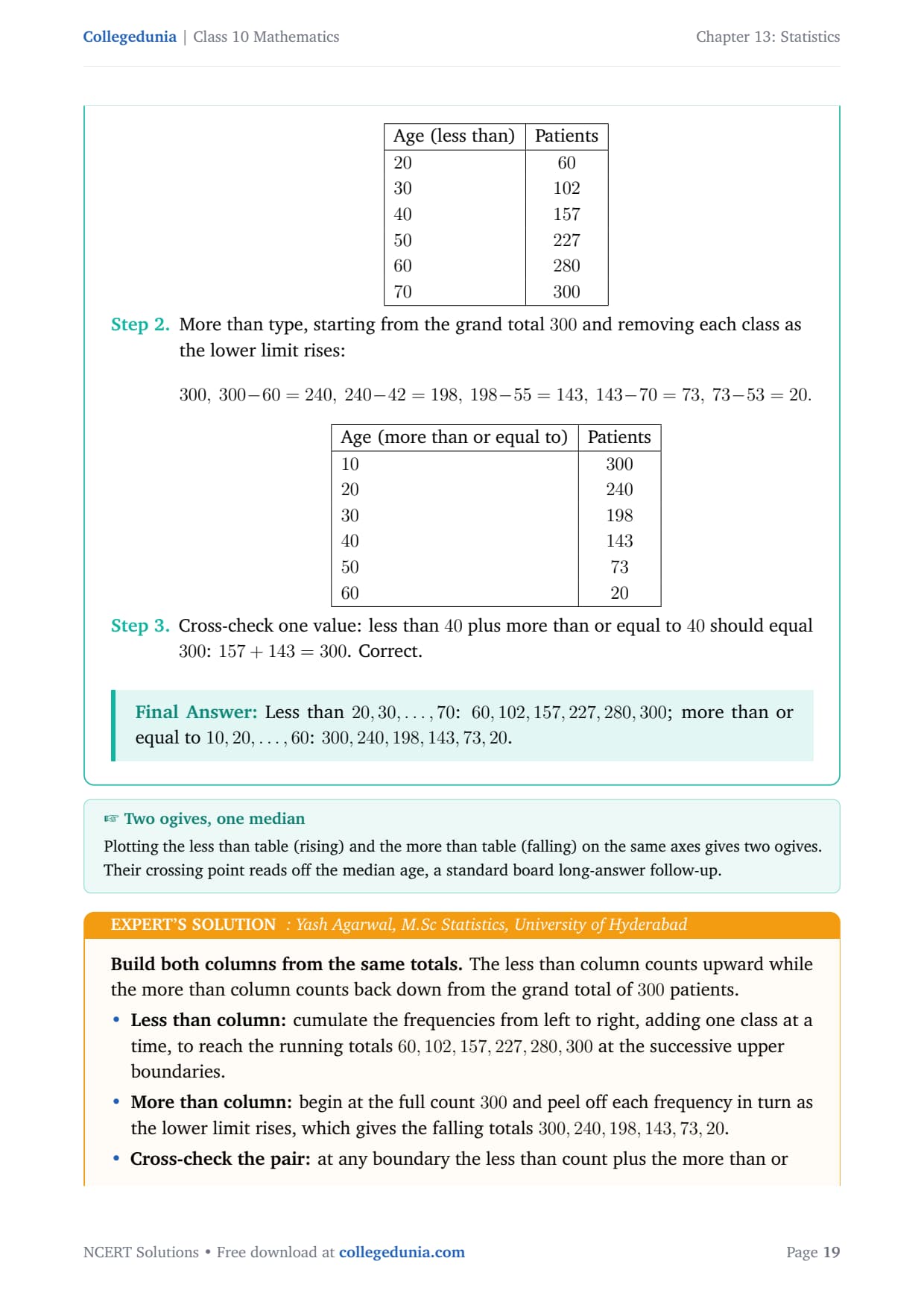
60, 60+42=102, 102+55=157, 157+70=227, 227+53=280, 280+20=300.
More than type, starting from the grand total 300 and removing
each class as the lower limit rises:
300, 300-60=240, 240-42=198, 198-55=143, 143-70=73, 73-53=20.
tabular|l|c|
Age (more than or equal to) & Patients 10 & 300 20 & 240 30 & 198 40 & 143 50 & 73 60 & 20
tabular
Cross-check one value: less than 40 plus more than or equal to
40 should equal 300: 157+143=300. Correct.
Less than 20,30,,70: 60,102,157,227,280,300; more than or equal to 10,20,,60: 300,240,198,143,73,20.
YA
Yash Agarwal
M.Sc Statistics, University of Hyderabad
Verified Expert
Build both columns from the same totals. The less than column
counts upward while the more than column counts back down from the grand
total of 300 patients.
Less than column: cumulate the frequencies from left to
right, adding one class at a time, to reach the running totals
60,102,157,227,280,300 at the successive upper boundaries.
More than column: begin at the full count 300 and peel
off each frequency in turn as the lower limit rises, which gives
the falling totals 300,240,198,143,73,20.
Cross-check the pair: at any boundary the less than
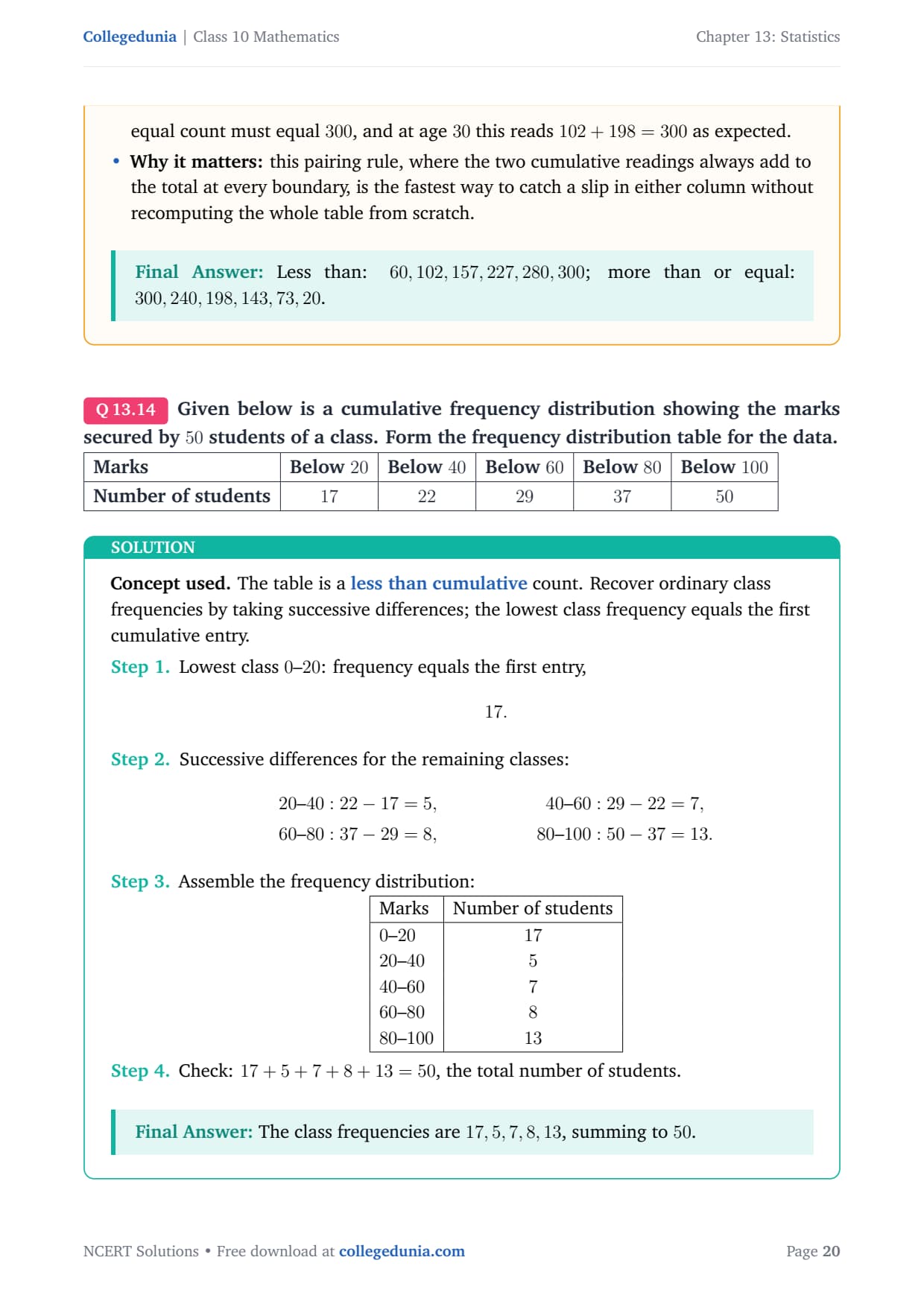
count plus the more than or equal count must equal 300, and at
age 30 this reads 102+198=300 as expected.
Why it matters: this pairing rule, where the two
cumulative readings always add to the total at every boundary, is
the fastest way to catch a slip in either column without
recomputing the whole table from scratch.
Less than: 60,102,157,227,280,300; more than or equal: 300,240,198,143,73,20.
Q 13.14
Given below is a cumulative frequency distribution showing the marks secured by 50 students of a class. Form the frequency distribution table for the data. [2pt]
tabular|l|c|c|c|c|c|
Marks & Below 20 & Below 40 & Below 60 & Below 80 & Below 100
Number of students & 17 & 22 & 29 & 37 & 50
tabular
Concept used. The table is a less than cumulative
count. Recover ordinary class frequencies by taking successive
differences; the lowest class frequency equals the first cumulative
entry.
Lowest class 0–20: frequency equals the first entry,
17.
Marks & Number of students 0–20 & 17 20–40 & 5 40–60 & 7 60–80 & 8 80–100 & 13
tabular
Check: 17+5+7+8+13 = 50, the total number of students.
The class frequencies are 17,5,7,8,13, summing to 50.
SK
Simran Kohli
M.Sc Mathematics, IIT Kanpur
Verified Expert
Difference the below column. The first entry stands on its own
while every later entry is just a gap between neighbours.
First class alone: since nothing lies below the lowest
mark, the opening cumulative total is also the first class
frequency, so the frequency of 0–20 is 17.
Gaps for the rest: each later class frequency is its own
below total minus the previous below total, which produces the
successive values 5,7,8,13 down the table.
Check the sum: adding everything gives
17+5+7+8+13=50, matching the class size, so no subtraction
slipped.
Why it matters: the wide classes of width 20 make the
below jumps look small, yet the opening class carrying 17 of the
50 students shows most marks are low, a shape that the
cumulative table hides until you difference it.
Frequencies 17,5,7,8,13 (total 50).
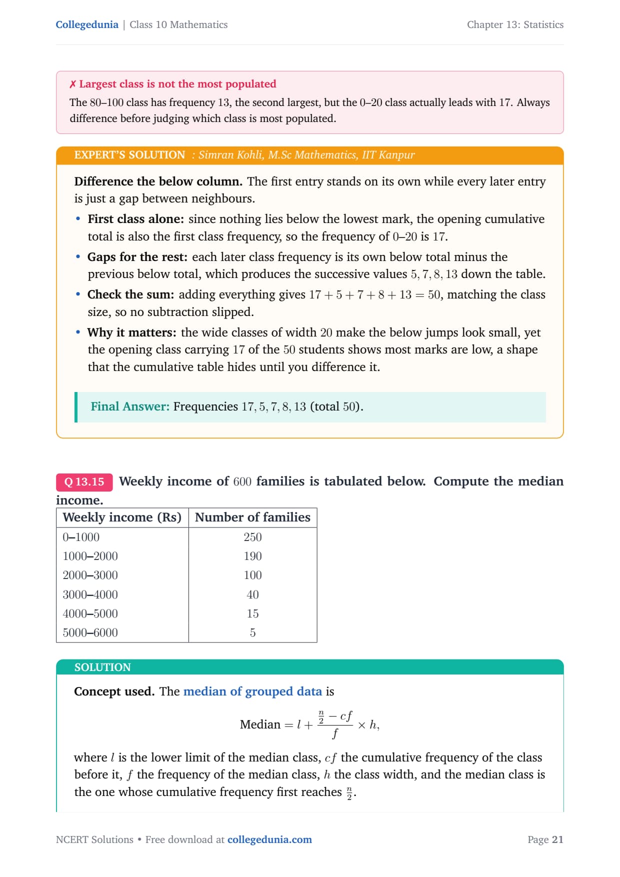
Q 13.15
Weekly income of 600 families is tabulated below. Compute the median income. [2pt]
tabular|l|c|
Weekly income (Rs) & Number of families 0–1000 & 250 1000–2000 & 190 2000–3000 & 100 3000–4000 & 40 4000–5000 & 15 5000–6000 & 5
tabular
Concept used. The median of grouped data is
Median=l+n2-cff× h,
where l is the lower limit of the median class, cf the cumulative
frequency of the class before it, f the frequency of the median class,
h the class width, and the median class is the one whose cumulative
frequency first reaches n2.
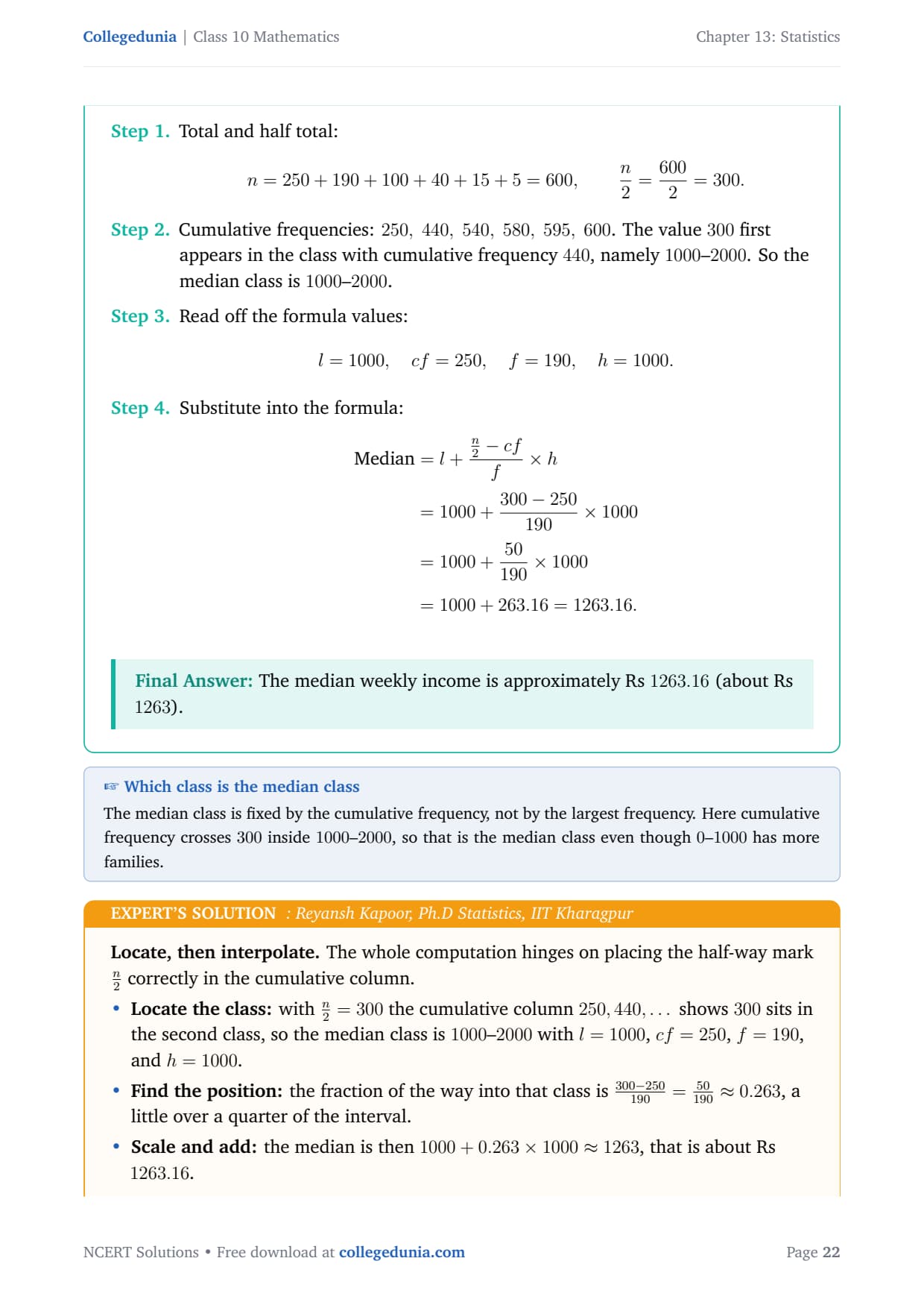
Total and half total:
n = 250+190+100+40+15+5 = 600, n2=6002=300.
Cumulative frequencies: 250, 440, 540, 580, 595, 600. The
value 300 first appears in the class with cumulative frequency
440, namely 1000–2000. So the median class is
1000–2000.
Read off the formula values:
l=1000, cf=250, f=190, h=1000.
Substitute into the formula:
MATH0
The median weekly income is about Rs 1263.16 (about Rs 1263).
RK
Reyansh Kapoor
Ph.D Statistics, IIT Kharagpur
Verified Expert
Locate, then interpolate. The whole computation hinges on
placing the half-way mark n2 correctly in the cumulative
column.
Locate the class: with n2=300 the cumulative
column 250,440, shows 300 sits in the second class, so
the median class is 1000–2000 with l=1000, cf=250,
f=190, and h=1000.
Find the position: the fraction of the way into that
class is 300-250190=50190≈ 0.263, a
little over a quarter of the interval.
Scale and add: the median is then
1000+0.263× 1000≈ 1263, that is about Rs 1263.16.
Why it matters: this median sits far below the top
brackets, reflecting that most families earn under Rs 2000, and
because the median resists the pull of a few high incomes it is
preferred to the mean for such skewed income data.
Median income ≈ Rs 1263.16.
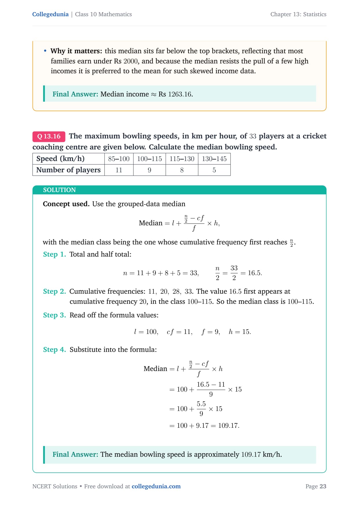
Q 13.16
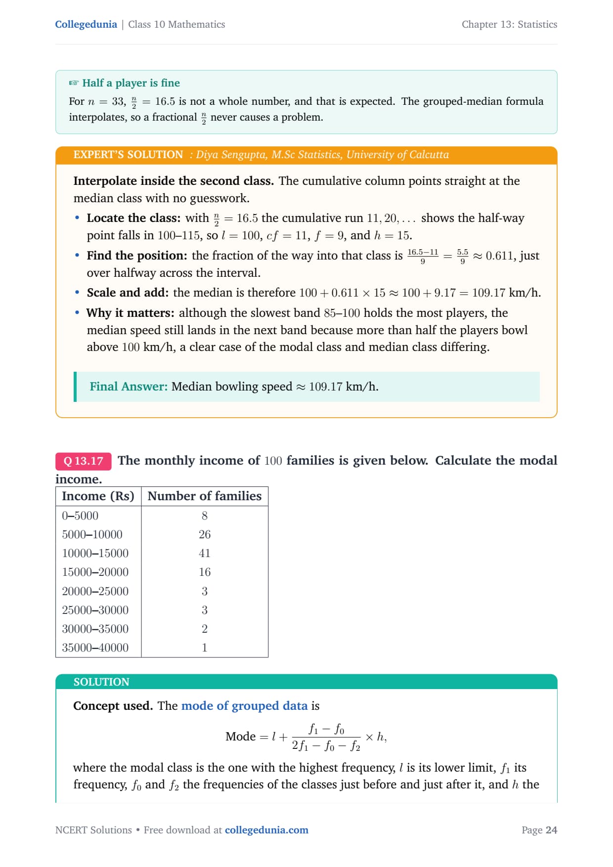
The maximum bowling speeds, in km per hour, of 33 players at a cricket coaching centre are given below. Calculate the median bowling speed. [2pt]
tabular|l|c|c|c|c|
Concept used. Use the grouped-data median
Median=l+n2-cff× h,
with the median class being the one whose cumulative frequency first
reaches n2.
Total and half total:
n = 11+9+8+5 = 33, n2=332=16.5.
Cumulative frequencies: 11, 20, 28, 33. The value 16.5
first appears at cumulative frequency 20, in the class
100–115. So the median class is 100–115.
Read off the formula values:
l=100, cf=11, f=9, h=15.
Substitute into the formula:
MATH0
The median bowling speed is about 109.17 km/h.
DS
Diya Sengupta
M.Sc Statistics, University of Calcutta
Verified Expert
Interpolate inside the second class. The cumulative column
points straight at the median class with no guesswork.
Locate the class: with n2=16.5 the cumulative
run 11,20, shows the half-way point falls in 100–115,
so l=100, cf=11, f=9, and h=15.
Find the position: the fraction of the way into that
class is 16.5-119=5.59≈ 0.611, just
over halfway across the interval.
Scale and add: the median is therefore
100+0.611× 15≈ 100+9.17=109.17 km/h.
Why it matters: although the slowest band 85–100
holds the most players, the median speed still lands in the next
band because more than half the players bowl above 100 km/h,
a clear case of the modal class and median class differing.
Median bowling speed ≈ 109.17 km/h.
Q 13.17
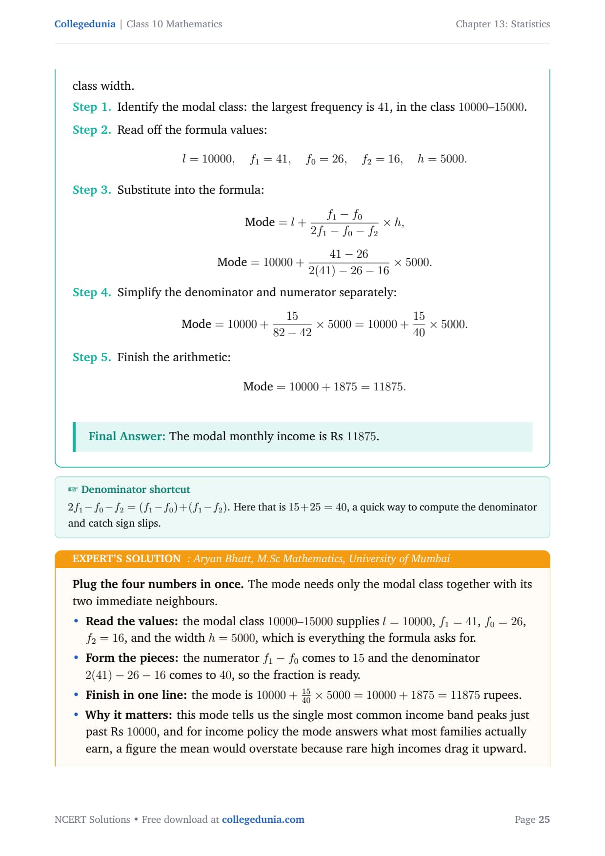
The monthly income of 100 families is given below. Calculate the modal income. [2pt]
tabular|l|c|
Concept used. The mode of grouped data is
Mode=l+f1-f02f1-f0-f2× h,
where the modal class is the one with the highest frequency, l is its
lower limit, f1 its frequency, f0 and f2 the frequencies of the
classes just before and just after it, and h the class width.
Identify the modal class: the largest frequency is 41, in the
class 10000–15000.
Read off the formula values:
l=10000, f1=41, f0=26, f2=16, h=5000.
Substitute into the formula:
Mode=l+f1-f02f1-f0-f2× h, Mode=10000+41-262(41)-26-16× 5000.
Simplify the denominator and numerator separately:
Mode=10000+1582-42× 5000
=10000+1540× 5000.
Finish the arithmetic:
Mode=10000+1875=11875.
The modal monthly income is Rs 11875.
AB
Aryan Bhatt
M.Sc Mathematics, University of Mumbai
Verified Expert
Plug the four numbers in once. The mode needs only the modal
class together with its two immediate neighbours.
Read the values: the modal class 10000–15000 supplies
l=10000, f1=41, f0=26, f2=16, and the width h=5000,
which is everything the formula asks for.
Form the pieces: the numerator f1-f0 comes to 15
and the denominator 2(41)-26-16 comes to 40, so the fraction
is ready.
Finish in one line: the mode is
10000+1540× 5000=10000+1875=11875 rupees.
Why it matters: this mode tells us the single most common
income band peaks just past Rs 10000, and for income policy the
mode answers what most families actually earn, a figure the mean
would overstate because rare high incomes drag it upward.
Modal income = Rs 11875.
Q 13.18
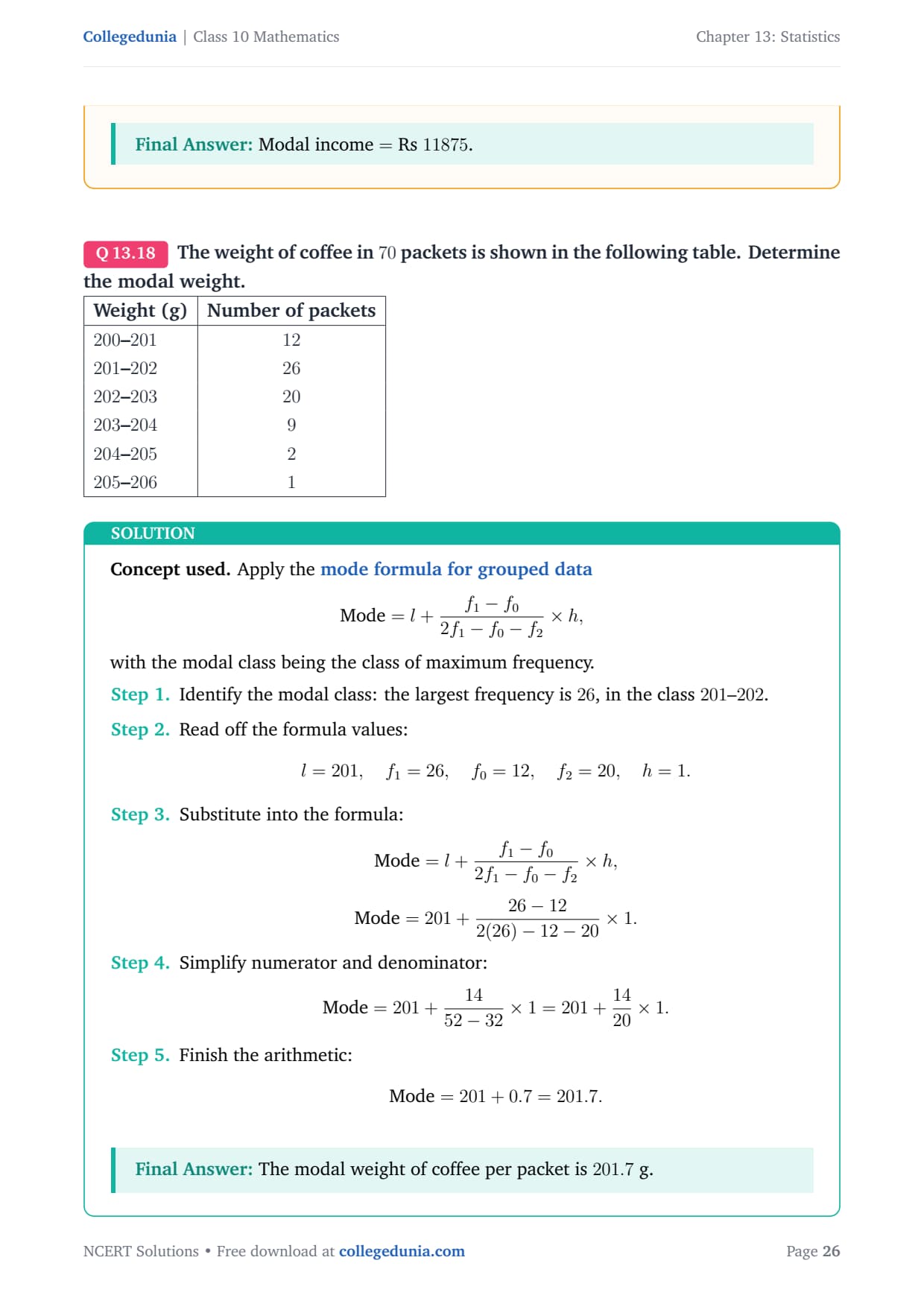
The weight of coffee in 70 packets is shown in the following table. Determine the modal weight. [2pt]
tabular|l|c|
Concept used. Apply the mode formula for grouped data Mode=l+f1-f02f1-f0-f2× h,
with the modal class being the class of maximum frequency.
Identify the modal class: the largest frequency is 26, in the
class 201–202.
Read off the formula values:
l=201, f1=26, f0=12, f2=20, h=1.
Substitute into the formula:
Mode=l+f1-f02f1-f0-f2× h, Mode=201+26-122(26)-12-20× 1.
Simplify numerator and denominator:
Mode=201+1452-32× 1
=201+1420× 1.
Finish the arithmetic:
Mode=201+0.7=201.7.
The modal weight of coffee per packet is 201.7 g.
PI
Pranav Iyer
M.Sc Statistics, University of Pune
Verified Expert
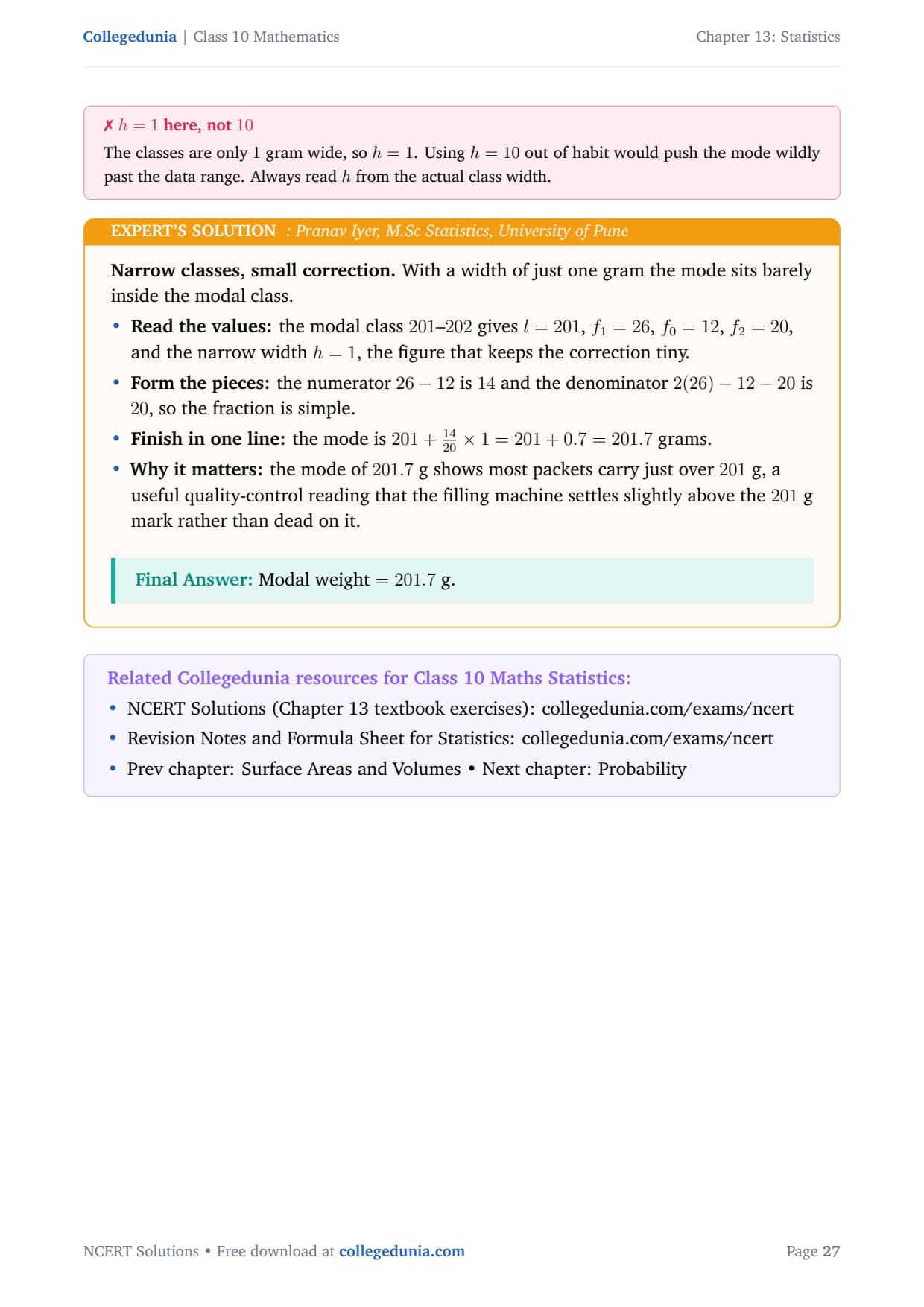
Narrow classes, small correction. With a width of just one gram
the mode sits barely inside the modal class.
Read the values: the modal class 201–202 gives
l=201, f1=26, f0=12, f2=20, and the narrow width
h=1, the figure that keeps the correction tiny.
Form the pieces: the numerator 26-12 is 14 and the
denominator 2(26)-12-20 is 20, so the fraction is simple.
Finish in one line: the mode is
201+1420× 1=201+0.7=201.7 grams.
Why it matters: the mode of 201.7 g shows most packets
carry just over 201 g, a useful quality-control reading that the
filling machine settles slightly above the 201 g mark rather
than dead on it.
Modal weight =201.7 g.
NCERT Exemplar Class 10 Maths Statistics Solutions: Frequently Asked Questions
Ques. Where can I download the NCERT Exemplar Class 10 Maths Chapter 13 Solutions for free?
Ans. You can download the NCERT Exemplar Class 10 Maths Chapter 13 Statistics Solutions PDF directly from this page using the red Download button above. The PDF is free and aligned to the 2026-27 CBSE syllabus.
Ques. How many problems are there in the Statistics Exemplar, and what types are they?
Ans. Chapter 13 has 31 Exemplar problems: 13 MCQs in Exercise 13.1, 6 fill-in-the-blank questions in Exercise 13.2, 7 short-answer computation problems in Exercise 13.3, and 5 long-answer application questions in Exercise 13.4. Problems cover mean by all three methods, median, mode, the empirical relation, and ogive-based questions.
Ques. What are the most important formulas for Class 10 Maths Chapter 13 Exemplar?
Ans. The key formulas are: Mean (direct method) = Σfx / Σf; Mean (assumed mean method) = a + Σfd / Σf where d = x - a; Mean (step deviation) = a + (Σfu / Σf) × h where u = (x - a)/h; Median = l + ((n/2 - cf)/f) × h; Mode = l + ((f1 - f0)/(2f1 - f0 - f2)) × h; Empirical relation: Mode = 3 Median - 2 Mean. The ogive intersection gives the median graphically.
Ques. What is the difference between a "less than" ogive and a "more than" ogive?
Ans. A "less than" ogive plots cumulative frequency (adding frequencies from the smallest class upward) against the upper class boundaries. It rises from left to right. A "more than" ogive plots cumulative frequency (adding frequencies from the largest class downward) against the lower class boundaries. It falls from left to right. When both are drawn on the same axes, the point where they intersect has an x-coordinate equal to the median of the distribution. This graphical method is an alternative to the median formula and is directly tested in CBSE board papers.
Ques. How is the Chapter 13 Exemplar harder than the NCERT textbook exercises?
Ans. The NCERT textbook has three exercises with direct formula applications to fully given frequency distributions. The Exemplar raises the level in three ways. First, Exercise 13.2 fill-in-the-blank questions test the empirical relation and ogive rules without a frequency table to work from. Second, Exercises 13.3 and 13.4 introduce two missing frequencies that require simultaneous equations using both the total frequency and the given mean. Third, Exercise 13.4 asks students to read the median directly from an ogive intersection and justify why that intersection gives the median value.
Ques. What is the most common mistake students make in Chapter 13 Exemplar problems?
Ans. The most common mistake is identifying the wrong class for median or mode. The median class is the first class where the cumulative frequency exceeds n/2, not the class with the highest frequency. The modal class is the class with the highest frequency, not the class containing the arithmetic mean. Writing a full cumulative frequency table before applying either formula prevents this error every time. The second most common mistake is forgetting to multiply by h in the step deviation method, giving a result near the assumed mean instead of the actual mean.
Ques. How much time should a Class 10 student spend on the Chapter 13 Exemplar?
Ans. Plan about 2.5 hours in total: roughly 25 minutes for the 13 MCQs, 15 minutes for the 6 fill-in-the-blank questions, about 40 minutes for the 7 short-answer computation problems, and 50 minutes for the 5 long-answer application questions, plus a revision pass on any question you got wrong. Students who write out the full frequency table (with all required columns) before touching any formula will work much faster and avoid the class-identification errors that slow down the computation exercises.








Comments